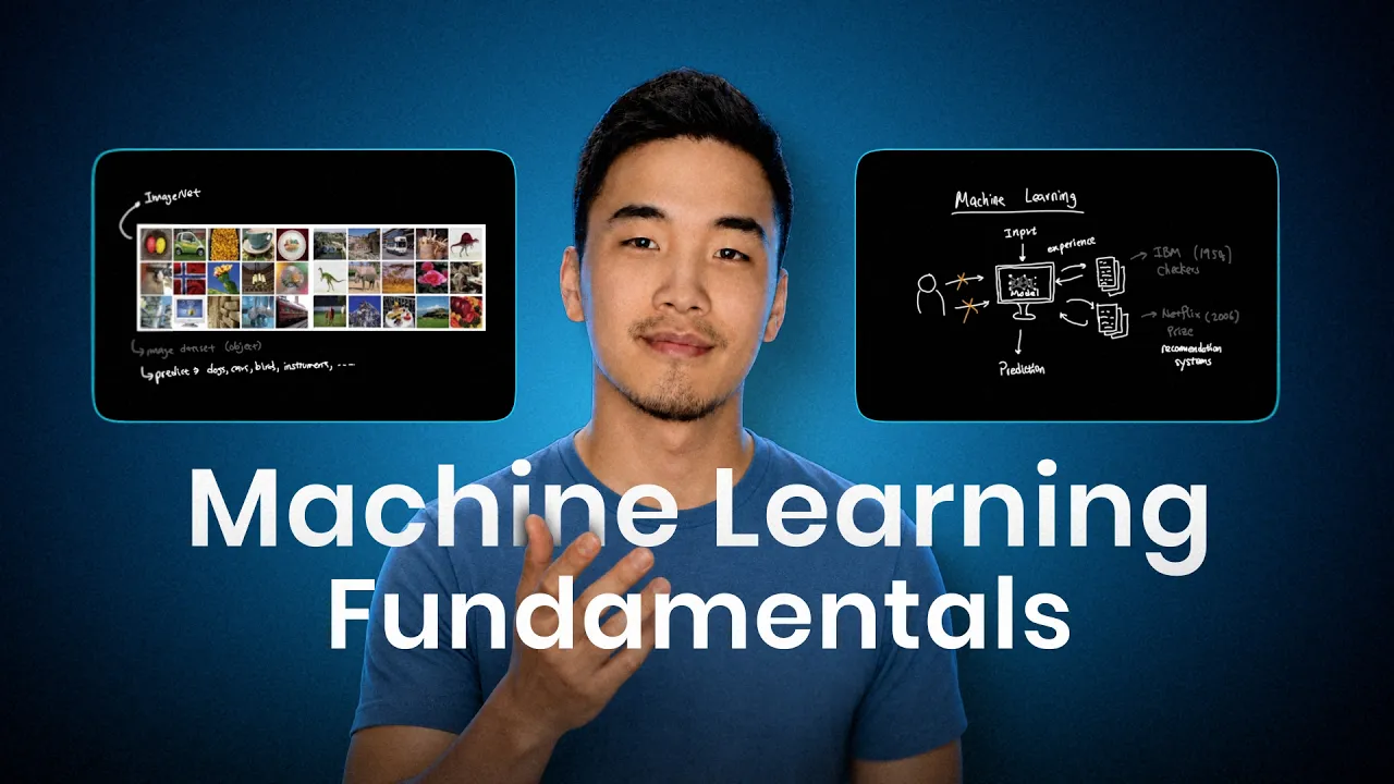
How Machine Learning Works, End to End (Full Basics) transcript
KodeKloud · @KodeKloud
Words
10,618
Runtime
1:00:28
Speaking pace
176wpm
Reading time
44min
176 words per minute, between the 160 25th percentile and the 181 median of 349 measured videos. That distribution comes from the 349-video hook study.
Opening (first 30 seconds)
Before we dive into the individual concepts, let's quickly look at the journey ahead. We'll start with the history of machine learning and define what machine learning actually is. Then we'll break down the core ingredients, data, features, labels, models, parameters, and weights. From there, we'll look at how models learn through training, loss functions, and gradient descent, and how we test whether we can perform well on new data. We will then compare different types of machine learning including supervised and unsupervised learning classification and regression. Finally,
88 words, the words spoken in the first 30 seconds at 176 words per minute.
Sentence shape
| Measure | This transcript |
|---|---|
| Sentences | 804 |
| Average words per sentence | 13.2 |
| Longest sentence | 43 words |
| Questions asked | 12 |
| Sentences containing a number | 57 |
Most used terms
- model247
- data98
- learning82
- training74
- house62
- prediction62
- price55
- loss51
- example46
- actually45
- parameters42
- models39
Filler phrases
113 in total: like 61 · actually 45 · kind of 4 · basically 2 · right? 1.
A literal whole-word count of the same phrase list the Prepublish browser extension uses, so a phrase inside another word is not counted and a phrase used in its ordinary sense still is. It is a count and not a judgement.
What this transcript is
Every word below is the caption track YouTube publishes for this video, pulled from the video itself and reproduced unchanged. It is not Prepublish's writing, not a summary, and not a re-transcription: it is the video's own published captions. English captions, generated automatically by YouTube, in the video’s original language. Source: the video on YouTube. A channel that would rather this page did not exist can ask for its removal through the contact page, and it is removed.
Transcript
Before we dive into the individual concepts, let's quickly look at the journey ahead. We'll start with the history of machine learning and define what machine learning actually is. Then we'll break down the core ingredients, data, features, labels, models, parameters, and weights. From there, we'll look at how models learn through training, loss functions, and gradient descent, and how we test whether we can perform well on new data.
We will then compare different types of machine learning including supervised and unsupervised learning classification and regression. Finally, we'll bring everything together with neural networks. Explain how models like GBT are actually trained. Explore evaluation metrics and finish with some of the modern approaches shaping AI today. By the end, you should understand the complete journey from raw data to a trained model making useful predictions.
So, let's get started. Most people think machine learning started with asking Chacha Piti to finish writing my essay for school. But the idea of making machines learn is much older than that. Long before we had AI assistants writing code, generating images, or finishing my school work, researchers were already asking a much simpler question. Can a machine improve at a task without a human explicitly programming every single use?
This question actually goes all the way back to early days of computing. In 1950, Alan Touring asked whether machines could imitate human intelligence. A few years later, in 1956, the Dartmouth workshop helped establish artificial intelligence as a formal field of research. Around the same era, Arthur Samuel at IBM was working on a checker program that could improve through experience. But early computers were extremely limited.
So, a lot of early AI was built around rules, logics, and search. Humans would try to encode intelligence manually. If this happened, then do that. If that happens, then do this. If the board look like this, make this move. If the user says this, return to the answer. And to be fair, this approach led to some very impressive systems. One of the famous examples was IBM's Deep Blue. In 1997, Deep Blue defeated Gary Kasparov, the world's chess champion at the time.
This was a massive moment for AI, but Deep Blue was still a very specialized system built on one narrow domain. It could calculate chess positions better than any human, but it could not suddenly explain why your code is throwing an error on line 47, for example. That kind of approach works well when the environment is clean and well- definfined. Chess has clear rules, clear boards, and legal moves and a clear win condition.
But most real world problems are not like chess. Recognizing faces, translating language, detecting spam, recommending videos, and driving a car are much messier problems. You can't realistically write every possible rule by hand. This is where machine learning becomes important. Instead of telling the computer exactly what to do, we give it examples and let it learn patterns from the data. Traditional software is mostly about humans writing the rules.
Machine learning is about creating a system that can learn useful patterns from the examples. One of the most important ideas in the industry was neural networks. Early neuronet networks were inspired by the human brain. The basic idea was that you could maybe take inputs, apply weights to these inputs, pass them through a function, and then produce an output. But for a long time, neural networks were hard to train. The hardware was really weak.
And the models were too small to do anything truly impressive. The idea was powerful but the world did not yet have the right combinations of algorithm data and the compute to actually work it at a scale. One major breakthrough did come through around 1980s when back propagation became popularized. Back propagation gave neural networks a practical way to trace errors backwards through the network and update the weights.
In simpler terms, the model could make a prediction, measure how wrong it was, and adjust itself to be less wrong next time. Even then, neural networks did not immediately take over the world. Training large models required a lot of computation for a long time and computers were not very powerful enough back then to make these systems useful at scale. Then in 2012, everything changed. A neural network called AlexNet won the imageet image classification competition using GPUs.
And this became one of the major breakout moments for deep learning. Neuronet networks were not new, but the ingredients finally came together. More data from the internet, better architecture, and GPUs that could actually train these models much faster. From there, deep learning started to take over computer vision, speech recognition, translation, recommendation systems, and eventually language models. And a few years later, AlphaGo combined deep neural networks, reinforcement learning, and search to beat one of the best Go players in the world.
This mattered because go is much harder to brute force than chess. So the system needed a more learning based approach that are shown here. Then in 2017, the transformer architecture was introduced and this became the key building blocks behind modern large language models and eventually led to the wave of AI systems that we use today. So if the history of AI is this shift from handwritten rules to systems that can actually learn from examples, the next thing we need to understand is what it actually means for machine to actually learn.
Machine learning is a way to build software where systems learn patterns from the data instead of relying on rules written by humans. In traditional programming, a developer writes the instruction directly. You give the computer an input, the program follows the rules and then it gives you the output. For example, if you wanted to check whether someone is old enough to access a website, you don't really need machine learning.
You can just write a simple rule. If the user is 18 or older, allow access. If they're younger than 18, block access, and the logic is pretty clear and predictable and easy to write. But some problems are not that very clean. Imagine trying to write rules for detecting spam emails. You can start with simpler rules like if the email contains keywords like free money, mark it as a spam. If the email also has too many links, also mark it as a spam.
If the sender looks suspicious, mark it as a spam. But spammers change their wording. Normal emails sometimes contain links and not every suspiciouslook email is actually a spam. This is the type of problem where machine learning actually becomes useful. Instead of trying to manually write every single rule possible, we collect examples and let the system learn useful patterns from them. This idea goes back to Arthur Samuels checker program in IBM in the 1950s.
The point was not just to make a computer follow the rules of checkers. The point was to build a program that could improve through experience. A more modern systems is Netflix prize. In 2006, Netflix launched a competition to improve its recommendation system. The goal was not to handwrite rules for every viewers in every movie. The goal was to use past ratings to predict what the rating of the user might actually give to a movie that they hadn't watched yet.
In machine learning, we usually train something called a model. A model is part of the system that takes an input and produces a prediction. For Netflix example, the input might be information about the user, a movie, a pass rating, and the prediction is how much the user might actually like the movie in the end. And over the years they have refined their machine learning model. So you never leave their platform and binge all seasons of the office in one weekend.
So a simple way to think about machine learning model is this. Input goes in, model does some math and prediction comes out. The important difference is that we don't manually program every detail of that math. During training, the model looks at many examples and adjusts its internal values called parameters or weights. So the prediction improve. You can think of these as knobs inside the model that are tuned during learning.
So when we say a machine learns, we don't mean it understands the world like human. We mean its parameters change so it performs better at a specific task. It is also important to know that machine learning is not just one algorithm or one type of model. It is a broad field. Some machine learning models are simple like linear models or decision trees. Others are more complex like neuronet networks or large language models.
Chhattet is one modern example of machine learning. So in one sentence, machine learning is about using data to train models that can make useful prediction on new inputs. And because machine learning is about learning from examples, the next thing we need to define is basic ingredients of those examples, data, features, and labels. Now that we know that machine learning is about learning from examples, we need to define the basic ingredients of those examples.
The first is data. Data is the raw material the model learns from. It could be emails, images, videos, audio clips, transaction records, medical scans, sensor readings, or rows in a spreadsheet. But for simple example, let's use housing prices as an example. House price prediction is a classic beginner machine learning example. Kaggle's house prices advanced regression techniques. competition uses Ames housing data set with 79 explanatory variables describing homes in Ames Iowa and asks people to predict the final sale price.
Imagine we have a spreadsheet of homes that were sold in the past. Each row represents one house. Each column describes something about that house like square footage, number of bedrooms, neighborhood, lot size, year, or whether it has a garage. That full spreadsheet is the data set. Each row is one example, sometimes called a sample or training example. It is one piece of past data that the model can learn from. The columns that describe the house are called features.
A feature is an input variable that the model uses to make a prediction. In a house price, for example, the features are details about the home. The values that we want the model to predict is called a label or target. For house prices prediction, the label is a sale price. So the setup is this. The model looks at a feature of a house and tries to predict the label which is the price. This is a basic structure of supervised machine learning.
Supervised means the model is learning from examples where we already know the correct answer. We're basically saying here are what the house look like and here is what it's sold for. Now learn the pattern. Labels are important but they are not always available. Sometimes you have a data set without clear answers attached to each examples. In those cases, the goal may not be to predict a known label, but to discover patterns or structure about the data.
That is where unsupervised learning comes in, which we'll talk about later. Another important idea is feature engineering. Feature engineering means creating or transforming features so the model has better information to learn from. For example, the raw data set might give us the year of a house that was built in, but the model may learn more easily if we want that to turn into an age of the house. Or maybe we combine bedrooms and bathrooms into a total rooms feature.
The goal is not to cheat. The goal is to represent information in a way that makes useful patterns easier for the model to find. Features can also come in different forms. Some are numerical like square footage or age. Others are categorical, which means they represent categories like neighborhood or house style. This matters because models usually work with numbers. So categorical features often need to be converted into a numerical format before the model can use them.
That conversion is part of the data preparation. And data preparation is a huge part of machine learning because the model is only as good as the information that it learns from. If the price and the data set are wrong, the model learns from bad answers. If important details are missing, the model may not have enough signal. If data only comes in from one type of home or one city, the model may not actually work well from somewhere else.
This is connected to data distribution. A data distribution is basically the pattern of examples that the model sees during training. If real world data looks something very different from the training data, the model's prediction can get worse. For example, if you train a model only in suburban homes, it could struggle to price a New York shoe box where 3,000 a month gets you a closet with maybe some natural light. The model did not learn housing in general.
It learned from specific distribution of examples we gave it. This also connects to bias. Bias does not always mean someone intentionally made the model unfair. Sometimes it means a data set is incomplete, skewed, or not representative of the real world the model will be used in. That is why people say garbage in, garbage out. Better data usually leads to better models and bad data can make even a powerful model perform poorly.
But now it's time to try your first lab. First of all, you don't need to worry if you're not feeling confident for the lab because labs come with a lot of hints and solutions. In this lab, you'll get a raw data set of 300 house sales and data set has real problems in it. One house has no sale price and another house appears twice. You'll drop those bad rows, turn the year build column into the house age, and convert the neighborhood names into numbers a model can actually do math on.
By the end, you have the exact file the model can actually train on. So, go give this lab a try. Having the data is only the starting point. The model still has to learn from it first and then later use what it learned on new examples. These are two very different phases, training and inference. Once we have collected the data, done some feature engineering and identified the labels, the next thing to understand is that machine learning is usually happening in two separate phases.
Training and inference. Training is the learning phase. Continuing with our housing prices example, training is when we show the model past home where we already know this final sale price. The model looks at features of each house, makes a prediction, compares the prediction to the real price, and then adjusts itself so it can do better next time. So maybe the model sees a house and predicts that it should sell for $700,000, but the actual sale price was $800,000.
During training, the model is allowed to see that answer. You can use the difference between the prediction and the real label as feedback. A simple way to think about this is practice questions with an answer key. When you are studying, you try the question, check the correct answer, and see where you actually got wrong and then adjust your understanding about the problem. Training works in a similar way. The model makes a guess, checks how it was wrong, and then updates itself.
We'll talk about how wrong part later when we get into loss functions. And we'll talk about the update itself part when we get into gradient descent. But for now, the important idea is that training is the phase where the model is actually learning. Inference is different. It's the usage phase. This is when we take a trained model and give it a new input that we don't actually know the answer for. So after the house price model have been trained, we might give it a new listing.
The model sees the features at the model and then predicts a price. But this time there's no answer key attached. The model isn't comparing the prediction to a real sale that happened in the past. It's just using the patterns that it had learned and actually making a prediction. This is important distinction because people often assume that when we use a model like talking to Chachi for example, it is also learning at the same time.
But this is not always true. In most machine learning system, using a model is simply inference. If a real estate website predicts a price of a home, the model is not necessarily retraining itself every time someone views a listing. It is usually using a model that was already trained earlier. So training is when the model learns from examples with known answers and inference is when that trained model makes prediction on new examples.
But saying the model updates itself during training is still a little vague. If something is changing inside the model, we need to understand what that thing actually is. This brings us to models, parameters, and weights. When a model learns, it is not rewriting itself like a programmer editing code. What changes are internal values that the model uses to turn inputs into predictions. At a high level, a model is part of a machine learning system that takes features as inputs and produces a prediction as outputs.
In our housing price example, the model takes information about a house and predicts that sale price. Under the hood, the model is doing math. Let's start with the simplest possible version. Imagine we only use one feature, square footage. A basic model might look at something like this and say predicted price equals weight time square footage plus bias. Or written more mathematically, prediction equals wx plus b. Where yhat means the predicted value.
In our case, this is the predicted house price. X is the input feature like square footage, W is weight and B is bias. This bias term has nothing to do with the data set bias we discussed earlier. They happen to use the same word. But here bias simply means a learned baseline offset in the model's equation. The weight controls how much the feature actually matters. If the square footage weight is high, the model is saying that every extra square footage adds a lot to the predicted price.
If the weight is lower, then the model is saying that square footage matters less. The bias is the baseline offset. It shifts the whole prediction up or down. In a house pricing model, the bias might represent the fact that even before we account for square footage, a home has some baseline value because of land, location, and a housing market. For example, the model might learn something like this. Predicted price equals 400* square footage plus 100,000.
So for a 1500 ft² home, the model were predicted something like this. 400 * 1500 + 100,000 equals 700,000. That is obviously simplified, but it shows you some idea. The model is not memorizing every single house. It is learning values that actually help turn inputs into predictions. Of course, real house price models usually is more than one feature. We might use square footage, number of bedrooms, age of the house, neighborhood, lot size and many other variables and many other variables.
So the equation becomes more like predicted price equals w sub1 * x1 plus w sub 2 * x2 and so on and plus b. Each features gets its own weight. One weight might control the effect of the square footage. Another might control the effect of the house. Another might control the effect of location. These learned values are called parameters. A weight is one type of a parameter. A bias is also a parameter. And more generally, parameters are internal values that the model learns during training.
So when we say that a model is learning, we usually mean its parameters are changing. Different types of model represent this prediction function in different ways. A linear model uses weights in a simple equation. A decision tree makes predictions by asking sequence of yes or no questions. Neural network uses layers of weights to learn more complex patterns. We'll get into neural networks later, but for now, the important idea is that every model has some structure it uses to turn inputs into prediction.
This can be very small or extremely large depending on the model. A simple linear model using 79 variables from Kaggle's house price data set might have something around 80 parameters, one weight for each variable plus one bias term. In practice, after converting categorical features like neighborhood or house style into numbers, that could become a few hundred parameters. Then at the other extreme, a modern AI models that have billions of parameters like GBT3 has 175 billion parameters.
Meta Lama 2 models is released in 7 billion, 13 billion, 70 billion parameters in sizes. The scale is completely different, but the core idea is still the same. Parameters are the learned internal values that shape the model's predictions. To wrap up, a model is a prediction function and parameters are learned values inside that function that gets adjusted during training. But just having parameters does not mean they are good parameters.
The model still needs to learn a way to measure whether its prediction was right or wrong. That brings us to loss functions. At this point, we know that a model makes predictions using parameters, and training is a process where those parameters are adjusted. But there's still a problem. How does the model know if the parameters are any good? Continuing with our house price example, imagine the model predicts that a home will sell for $700,000, but the real sale price was $800,000.
As humans, we can immediately tell the model was wrong. But the model needs something more precise than just wrong. It needs a number that tells how bad the prediction actually was. That is what a loss function does. A loss function measures how far off a model's prediction is from the correct answer. The lower the loss, the better the prediction. For a house price model, a simplest place to start is the error. Error equals predicted price minus actual price.
So if the model predicted $700,000 and the house actually sold for $800,000, the error is $700,000 minus $800,000 which is minus100,000. So the model is off by $100,000. But using raw error by itself can create a lot of problems. If one house is under predicted by 100,000 and another house is overpredicted by 100,000, these errors can actually cancel each other out. The average error might even look closer to zero even though the model is making big mistakes.
So one common approach is square the error. For one example, the loss can be written something like this. L equals the square root of Yhat minus Y. Here the Yhat is the model's prediction. Y is the real label and the L is a loss. In our house price example, Yhat would be the predicted price and Y will be the actual sale price. If the model is off by a 100,000, the squared error is that very large number. The exact number here is less important than the actual idea.
The bigger mistakes gets punished more. This is useful because we do not want the model to treat a $5,000 mistake as the same as a $100,000 mistake. Squaring the error makes the errors stand out a lot more. Of course, a model is not trained on one house. In the Kaggle house price data set, the training set has 1460 homes. So instead of looking only at the loss of one prediction, we usually care about average loss across all those examples.
For house price prediction, one common loss function is called mean squared error or MSE. Mean squared error means we take one squared error for each example, then average them together. So if the model predicts prices for thousands of houses, MSE gives us one number that summarizes how wrong the model is across all those predictions. This number becomes the model's feedback signal. If the loss is high, the model's predictions are bad.
If the loss gets lower during training, the model is usually improving. Different problems can use different loss functions. For house prices, squared errors make sense because we are predicting a number. But if we were predicting categories like spam or not spam, we'll be using a different kind of loss. The loss function depends on the task. To summarize, a loss function turns prediction error into a number the model can actually optimize during training.
It gives the model a feedback signal. So training is not just guessing randomly, but trying to make that loss smaller over time. But measuring the loss is only half of the story. The model now knows how trash its prediction was, but still needs a way to change the parameters so that the loss gets smaller. That brings us to gradient descent. Now that we have a loss function, we have a way to measure how wrong the model is.
But measuring the problem is not the same thing as fixing it. The model still needs a way to change its parameters so the loss gets smaller. That is where gradient descent comes in. Gradient descent is the process of updating the model's parameters in the direction that reduces the loss, which usually means improving the model's performance on the training data. To understand this idea, imagine a ball is sitting on a hill.
The height of the hill represents the loss. A higher point means the model is making worse prediction. A worse a lower point means the model is making better prediction. The goal is to get the ball roll downhill towards the lowest point it can find. In machine learning, the model's current parameters are like the ball's current position on the hill. The loss function creates a surface on the hill. And gradient descent is the method that tells the model which way to move.
This is where the word gradient comes in. A gradient tells us the slope of the loss function at the model's current position. More practically, it answers questions like if we change this weight a little bit, does the loss go up or down? And by how much? For example, in our house price model, maybe we have a weight for square footage. If increasing that weight makes the model prediction worse, the gradient tells us that.
If increasing the weight makes the prediction better, the gradient also tells us that as well. The important thing is that the gradient points in the direction where the loss increases the fastest. So if you want to make the loss smaller, we want the opposite direction. That is the descent part of the gradient descent. The basic update rule looks something like this. New weight equals old weight minus learning rate times gradient or written more mathematically like this where w is the weight that we are updating.
The gradient tells us the direction and the steepness of the loss and alpha is a learning rate. In learning rates controls how big of the step the model takes each time to update its parameters. If the learning rate is too small, the model may improve, but training can be painfully slow. It is taking only tiny bits of steps down the hill. If the learning rate is too large, the model might overshoot. Instead of moving smoothly towards a lower loss, it can jump back and forth and fail to settle on a good place.
So training is not just about knowing the right direction. It's also about taking the right size step. Going back to our house price example, maybe the model starts assuming that each extra square footage adds about $400 to the house price. But after looking at many homes, calculating the loss, and checking the gradient, the model might adjust that weight. It might go from $400 per square foot to $45 per square foot, then $48 per square foot, then finally $410 per square foot.
The model is not magically finding the perfect answer in one step. It is making small updates over and over again, each time trying to reduce the loss. But in practice, the model does not process every house in training data set all at once. Instead, the data is divided into smaller groups called batches. The model makes predictions for one batch of the house, calculates the loss across that batch and then updates its parameters before moving on to the next batch.
Once the model has worked through every batch on the training set, it has completed one full pass in data set. This is called an epoch. Training usually runs for many epochs, meaning model sees the full data set multiple times and continuing refining its parameters along the way. So the training loops look something like this. The model makes a prediction for a batch. The loss function predicts how wrong those predictions were.
Gradient descent uses the gradient to update its parameters. Then the model moves to the next batch and repeats the process. After every batch has been processed, one epoch is completed. Then the next epoch begins. Over many batches, updates and epochs, the parameters become better tuned to that data. This is what we mean when we say the model is learning. It is not learning by memorizing every single house. It is learning by adjusting its parameters so that overall loss becomes smaller.
To summarize, gradient descent is a method that turns the loss function into action. The loss tells us the model how bad it predictions really is and gradient descent tells the model how to update its parameters to make that loss smaller. It's time for the next lab. In this lab, you'll be training the algorithm yourself. The model is one small formula with two knobs and you'll edit those knobs by hand. Run the predictions and watch the error respond until you find a good fit.
Go give it a try. This point the model has a way to improve during training. But we only have talked about improving the examples it has already seen. The real goal is not just to perform well on training data. The real goal is to make good predictions on new examples. That is why we need to separate our data into train validation tests. At this point, the model has a way to improve during training. It can make prediction, calculate the loss, use gradient descent to update its parameters and repeat that process many times.
However, improving the training data is not the same as improving in the real world. It is like gathering a perfect score on Dualingo, then never speaking to waiter in French in France. In our house price example, imagine we train the model in a data set of past home sales. If we only care about doing well on that exact data set, the model could start learning patterns that are too specific, it might pick up random quirks in the training data and instead of learning patterns that apply to house more generally.
This is called overfitting. Overfitting happens when a model learns the training data too closely. May look good during training, but when we give it a new house it has never seen before, the prediction can be much worse. A simple analogy is memorizing practice questions before an exam. If the real exam has the exact same question, you might do well. But if the exam asks new questions that test the same concepts, memorization will fall apart.
Machine learning has the same issue. We do not just want the model to memorize a house price in the data set. We want it to generalize, meaning we wanted to make good predictions on new homes as well. This is why we split the data into different sets. The training set is the data that the model actually learns from. These are examples used to update the model's parameters. In the house price example, the training set will be a large chunk of past home sales.
The model sees the features, predicts the price, compares its prediction to real sale price, and updates itself. The validation set is used while we are building the model. It helps us check how well the model performs on examples it is directly training on. For example, if the model keeps getting better on training set but starts getting worse on validation set, that is a warning sign. It may be overfitting. The model is becoming too specialized to training examples and losing its ability to generalize.
The test set is a final check. This is the data that we hold back until the end after we have trained the model and made our major decisions. The test set is supposed to estimate how the model will perform on truly unseen data. So the basic idea is this. Training set means learn from this. Validation set means tune and check during development. Test set is final evaluation. A common rule of thumb is something like 70% training, 15% validation, and 15% test.
Another common split is 80 for training, 10 for validation, and 10 for test. There's no perfect split for every problem. If you have a lot of data, you can afford to hold out more for validation and testing. If you have smaller data set, you may want to keep the data for training. In some cases, people use techniques like cross validation where the data is split multiple ways to get more reliable estimate of performance.
The principle is simple. Do not judge the model only on examples it learned from. There's also one important mistake to avoid. Data leakage. Data leakage happens when information from the validation or test set actually sneaks into training. If that happens, the model may look better than it really is because it has indirectly seen information it was not supposed to have. In our house price example, this could happen if we accidentally include a feature that gives away the final sale price or if the same house appears in both training and test data.
The model might look accurate, but the evaluation would not be trustworthy. So to summarize, train, validation, and test sets exist because the goal is not just to reduce training loss. The goal is to build a model that generalizes on new examples. Time for one more lab. In this lab, you'll split your data into training, validation, and test sets. Then you'll train a decision tree with no limits and watch it score almost perfectly on training and terribly on validation because it memorized the houses instead of learning the patterns.
You'll fix that by setting limit on its depths. Then a colleague hands you a data set that scores suspiciously well and you'll figure out the leak by hiding inside in it. Go and try this lab. Once we understand how to split that data and evaluate generalization, we can zoom out and look at different kinds of machine learning problems. That starts with the difference between supervised and unsupervised learning. So far most of our examples have been supervised learning.
In our house price example, we have past homes. We have features about each home and we also have the correct answer. the final sale price. That is what makes it supervised. Supervised learning is when the model learns from examples where the answer is already provided. The model gets the inputs, makes a prediction, compares that prediction to a label, and then improves from that feedback. Another classic example is MNEST.
One of the most famous beginner data sets in machine learning. MNEST is a data set handwritten digits where each image shows a number from 0 to 9. The input is the image and the label is the correct digit. If the image shows a handwritten seven, the label is also seven. This became a common starting point for image classification because the task is simple to understand. Look at the image and predict the number. A larger and more famous image data set is imageet.
Imageet is a massive image data set organized around object categories and became especially important because of imageet challenge. Instead of predicting only the digits from 0 to 9, imagenet models had to classify images into many different categories like dogs, cars, birds, instruments, and other objects. The task changes, but the supervised learning structure is the same. The model is learning from examples where we always know what the correct output should be.
But not every data set comes with labels. Sometimes you have a lot of data but no clear answer key attached to each example. That does not mean the model's useless. It means that there's no label telling the model exactly what each example should be. This is where unsupervised learning comes in. Unsupervised learning is when the model tries to discover patterns, groups or structures in data without being given to the correct answer up front.
Going back to houses, imagine we have a large data set of homes, but we do not have the sale price. We just have the details about homes. An unsupervised model might still find patterns. It might group similar homes together. Small downtown condos, suburban family homes, older fixed uppers, luxury properties, and so on. The model is not predicting a known label. It is trying to discover structure in the data. A more relatable example is customer segmentation.
A company might have data about how users browse, buy, clicks, or watch content, but it may not have clean labels for what type of consumer each person is. An unsupervised algorithm can help group similar users together. For example, a streaming platform might discover one group of users who only watch professional darts, another who binge on Love Island, and another who puts on kids shows at 7:00 a.m. just to get 10 minutes of peace.
Nobody had to manually label these users ahead of time. The model finds a pattern in their behavior and groups similar users together. This technique is known as clustering. The idea is the same whether you're grouping viewers, customers, or houses. Find the natural groups hiding in the unlabeled data. So the main difference is this. Supervised learning asks, can we predict a known answer? Unsupervised learning asks, can we discover useful structure when there's no answer key?
So to wrap up, supervised learning uses labeled examples to learn a prediction task while unsupervised learning looks for patterns in data without labels. And since supervised learning is about predicting labels, the next useful distinction is what kind of label we are predicting. Sometimes a label is a number like a house price, other times a label is a category like spam or not spam. This brings us to classification and regression.
Now the work we covered so far is just the inner training loop where the model takes an input and makes a prediction to find out what the loss is to correct its parameters through gradients. This loop is how the model actually learns in the inner loop. Typically you also have this outer loop that experiments by choosing data features model types hyperparameters and eval to actually check on the validation set and change the external environment where the learning is hosted.
This is where you can actually adjust the learning rate and clean the data and add an edit feature to get the best result. This interplay between inner and outer loop is what helps you grow your understanding about machine learning as a larger system than a single training run and learn about how to mix different techniques as you go. Now that we know how supervised learning uses labeled examples, the next question is what kind of label are we trying to predict?
This is where we get the difference between classification and regression. Regression is when the model predicts a number. Our house price example is a regression problem because the label is a final sale price. The model looks at features about the house and predicts a number like $700,000, $850,000, or 1.2 million. Other regression examples include predicting rent, delivery time, temperature, revenue, or demand. In each case, the output is a number that can take many possible values, not one fixed category.
Classification is when the model predicts a category. A spam filter is a classification model because it predicts whether an email is spam or not spam. Mnest is also classification. The model looks at an image of a handwritten digit and predicts the number from 10 classes 0 to 9. So the simple difference is regression predicts values. Classification predicts classes. A common way to visualize this is with two graphs.
For classification, the model tries to draw boundaries between categories. This is a decision boundary. Points on one side belong to one class and points to other side belongs to another class. For regression, the model tries to fit a line or curve through that data. If house prices for example, you could imagine a square footage on the x-axis and sale price on the y-axis. The model is trying to learn relationship that helps predicts the price in the input features.
The output looks also different. The regression model usually gives you a number directly. Predicted house price equals $700,000. A classification model then gives us probabilities across classes. Spam could be 92% not spam could be 8% probability. Then the system chooses the class with the highest probability. This also affects how we train and evaluate the model. For regression, we usually care about how far the predicted number is from the real number.
For classification, we care whether the model gave enough probability to correct class. We'll see this again when we talk about neural networks and evaluation metrics. To summarize, regression is about predicting numbers and classification is about predicting categories. But whether we are predicting price, digits, or whether an email is a spam, the model still has to learn a relationship between inputs and outputs. Simple models can work for simple patterns, but complex problems often need more flexible models.
That brings us to neural networks. Now, we're at an exciting part. Neural networks are where a lot of ideas we have covered come together. Features, weights, biases, predictions, loss functions, gradient descent, classification, and regression buckle in. A neuronet network is a machine learning model made of many small mathematical units connected together. These units are often called neurons because the idea was loosely inspired by the brain.
The point is simply that many small connected units can work together to learn complex patterns. The idea goes back decades. Researchers have already been trying to model simple artificial neurons in the 1940s and by 1980s back propagation became a practical way to train networks with multiple layers. Neuronet networks feel modern today because data compute and training methods finally caught up. To understand how they work, let's start by looking at one artificial neuron.
A neuron takes in an input, multiplies each input by a weight, adds them together, and adds the bias. Sound familiar? The inputs are features. The weights decide how much each input actually matters. The bias shifts the results up or down. This is all a review from before. Mathematically, it looks something like this. Weighted sum equals W sub1 * X sub1 plus W sub2 * X sub2 + B. So if we had two inputs X sub1 and X sub2, the neuron would multiply each one by its own weight.
Add them together, add the bias, then produce an answer. One neuron by itself is limited. The real power comes in but from connecting many neurons into layers. A neural network usually has an input layer, one or more hidden layers, and an output layer. The input layer receives the data. The hidden layer processes the data and the output layer produces a final prediction. This is where activation function matters. If each layer only multiplied inputs by weights and added bias, stacking layers would not actually help very much.
The network would still behave like one big straight line model. An activation function is a simple mathematical rule applied inside the network that helps it learn more complex patterns. A common example is ReLU. ReLU turns a negative numbers into a zero and leaves a positive numbers alone. So, ReL minus 3= 0. ReLU 5= 5. That small step helps neural networks learn patterns that are not just straight lines. Let's make all this concrete with Mnest, the handwritten digit data set we were talking about earlier.
Each example is a small image of handwritten number from 0 to 9. The input is the image and the label is the correct digit. A neuronet network for Nest takes the image pixels as an input. Each pixel is just a number representing how dark or light that part of the image is. The network produces pixel values through its layers. Then the output layer produces a score for each possible digits. Those scores can be turned into probabilities like this.
The model chooses the digits with the highest probability. In this case, it predicts seven. This is a classification problem because the model is choosing one category from the fixed data set of classes. The process of data moving through the network to produce prediction is called forward pass. For MNEST, the forward pass is something like this. Pixels go in, layers process them, digit prediction comes out. So at this point, we have a basic structure.
A neural network is a stack of layers. Each layer has learned weights and biases. Activation functions help the network learn more complex patterns and forecast turns an input into prediction. But during training, the model also needs to learn from its mistakes. But how do we do that? Imagine the correct label is seven. But the model predicts one. Remember the loss function. We can use them to measure how bad that prediction was.
If the model gives high probability to the correct answer, the loss is low. If it gives low probability to the correct answer, the loss is high. Next, this is where back propagation comes in. Back propagation is the algorithm that works backwards through the network and figures out how each weight and bias contributes to the error. This matters because neural networks can have a lot of parameters. Instead of a few weights in simple model, they can have thousands, millions, billions, and even hundreds of billions that of learned values.
GPT4 was rumored to have around 1.8 a trillion parameters of values. Back propagation gives gradient descent the information it needs to updates those parameters. So the training loops look something like this. The model makes a prediction. The loss function measures the error. Back propagation works backwards to the network to calculate the gradient. Gradient descent uses the gradient to update the weights and biases.
Then the model tries again. Over many examples and many updates, the network gets better. For emnets, that means the model gradually learns patterns that help distinguish a three from an eight or four from a nine. This is one of the biggest reasons neuronet networks are powerful. They can learn useful features from raw data. Earlier we talked about feature engineering. In traditional machine learning, humans often design useful features by hand.
For house prices, we might create a feature like home age, total rooms, or distance from downtown. But neural networks can learn these internal features on their own. For images, earlier layers might learn simple patterns like edges, curves, or corners. Later layers might combine them into more useful shapes. For emnness, that might mean learning strokes, loops, or curves that actually identify each digit. That is also where the phrase deep learning comes from.
Deep learning usually means neuronet networks with many layers. The deep part does not mean the model is thinking deeply. It means the model has many layers of computation. For a long time, neuronet networks were promising but hard to train at scale. The idea existed but the hardware was much weaker. Data set was smaller and training large model was difficult. Then ingredients started to get better altogether. More data, better training methods and much more compute from GPUs.
One major breakthrough was a moment when AlexNet in 2012 was a deep neural network built for image classification and eventually performed extremely well on imageet challenge. ImageNet matters because it was a much larger harder image recognition benchmark than emnest. Instead of recognizing handwritten digits from 0 to 9, models had to recognize many kinds of real world objects. From there, neuronet networks became central to image recognition, speech recognition, translation, recommendation engine, and eventually large language models.
And this is important because GPT is also a neural network. It is obviously much larger and much more complex than a small MNET model that we just talked about. But the basic idea is still connected. Data goes in, it moves through layers and the model makes a prediction and the loss measures how wrong it was and training updates the parameters. The difference is the type of data and the scale. Instead of looking at pixels and predicting a digit, GPT looks at takes tokens and predicts what the next token should come next.
Now that we understand neural networks, we can talk about how large language models become useful assistance like chache BT. First, there's pre-training. This teaches the model broad language ability. Then there's post-training. This teaches instruction fine-tuning, which teaches a model how to follow instructions and methods like RLHF, which further shape the model's behavior so its answers are more helpful, safe, and useful to humans.
Let's start with pre-training. GPD does not work with raw text exactly the way that human reads it. Before the text goes into the model, it gets broken into smaller pieces called tokens. A token might be a word, part of a word, punctuation or smaller chunk of a text. But if you remember from earlier, model works with numbers, not words. Going back to the house price example, we had to convert categories like neighborhood into a numerical format.
Tokens go through the same idea at a large and a bigger scale. Each token gets turned into a long list of numbers called embedding. And tokens with similar meaning can end up with similar numerical representation. This is how a model can treat king and queen as related even though the letters actually look nothing alike. In the mnest example, pixels went in and the model predicted the digit. For GPT, token embeddings go in and the model predicts the next token.
During pre-training, the model looks at massive amounts of text and repeatedly tries to predict what token comes next. For example, if the text says the capital of France is and the model should learn what the next token should be like Paris. At the beginning, the model is bad at this. Its parameters are not really tuned yet. So, the prediction might be mostly wrong. But the training loop is the same as we already covered.
The model predicts the next tokens. The loss function measures how wrong it was. Back propagation calculates the gradients. Gradient descent updates the parameters and the model tries again. After doing this over and over across huge amount of text, the model starts to learn patterns. It learns grammar. It learns facts. It learns what explanation usually looks like. It learns how code is written. It learns the structure of language by trying to predict the next piece of text.
This is why next token prediction is most powerful than it sounds. The model is not manually programmed with every grammatical rule or every fact. It is learning patterns from examples. So pre-training gives GPT its broad language ability. But a pre-trained model is not automatically a helpful assistant. A model trained only to predict the next token is mainly learning how to continue the text. That is useful, but is not always the same as following a user's instruction.
Right now, it is just the ultimate autocomplete. For example, if you write, explain why Spider-Man is always broke. A raw pre-trained model might continue it like it found on a random web page. That is a continuation of text but is not really answering you directly. What if you want something more like this? This is where post- trainining comes in. One part of post-raining is instruction fine-tuning. Fine-tuning means taking a pre-trained model and training it further on examples of what actually we want it to do.
For an assistant, this means examples of user instructions and good responses. For example, if a user said this, by training on many examples like this, the model learns the pattern of being an assistant itself. So, instruction fine-tuning helps to turn a general language model into an instruction following model. But there's still another problem. There can be many possible answers to the same question. One answer might be technically correct but confusing.
Another might be clearer. One answer might be too long. Another might follow the user's request better. Some answers may be unsafe or unhelpful, but post- training does not stop an instruction fine-tuning. You can also include methods that further shape the model's behavior using feedback. One famous method is called RLHF, which stands for reinforcement learning from human feedback. The idea is that humans compare different model responses and signal which ones are better.
The model can then train to prefer answers that people rate more highly. So if the user asks explain why Superman is always broke and the model gives two possible answers, the human might prefer the one that is clear, shorter, and easier to understand. And that feedback helps train the model toward responses people actually find useful. This is the point of postraining. It is not always about predicting a likely next token anymore.
It is about shaping the model to give answers that are helpful, clear, and safe and aligned with what the actual users want. To summarize, pre-training teaches GPT broad language patterns by predicting the next token. Post-raining then shapes a model into useful assistant through instruction fine-tuning and feedback based methods like RHF. Underneath all of this, it is a neural network. Still data goes in, layers process them, predictions comes out, loss measures error, and training updates parameters.
The difference is the scale of the data, the size of the model, and the extra training stages that shape how it behaves. Now that we understand how GBT is trained, we need to know if the training actually worked. Let's see how we can measure this using different evaluation metrics. Once a model has been trained, we need a way to judge how good it actually is. An evaluation metrics is a number we use to measure models performance.
It helps answer questions like how close were the prediction. How often was the model right and does it actually work on new data. This connects back to train validation and test sets. We do not just care if the model did well on the examples if it trained on. We care if it generalizes. For regression problems where the model predicts a number, the main question is how far was the prediction from the real value. One common metric is mean absolute error or MAE.
MAE tells us how far off the model is on average. So if a house price model has MAE of $50,000, that means the predictions are off about $50,000 on average. Another common metric is mean squared error or MSE. MSE squares the errors before averaging them. So bigger mistakes get punished more. There's also RMS or root mean squared error which is the square root of MSE. This brings the error back into the original units.
For house prices, that means dollars. For regression, evaluation is mostly about measuring the size of the error. Classification is different because the model predicts the category. For emnest, the model predicts a digit from 0 to 9. For spam detections, it predicts spam or not spam. The simplest classification metrics is accuracy. Accuracy asks what percentage of prediction did the model get right. If an MNEST model correctly classifies 98 out of 100digit images, its accuracy is 98%.
But accuracy is not always enough. Imagine a spam filters where most emails are not spam. A model could predict not spam almost every single time and still look accurate even though it misses the emails we actually care about catching. This is why people also use prediction and recall. Prediction asks when the model predicts spam, how often is it right? Recall asks out of all the spam emails, how many did it catch? An F1 square combines the prediction and recalls one to another.
So for classification, we do not just care about if the model was right. We also care about what kinds of mistake that it actually was. Evaluation gets even harder with large English models. For housing prices, there's always a clear correct number. For emnness, there's always a clear correct digit, but for a chatbot, there can be as many good answers. If someone asks, "Explain neuronet networks simply," there's not one perfect response.
One answer might be shorter, another answer might be more detailed, and another might use a better analogy. So, language models are usually evaluated with a mix of benchmarks. Human preference ratings, factuality checks, coding tests, math problems, and real world use. But no single metric tells the whole story. A model can do well on a benchmark and still hallucinate facts. It can write fluent text but fail to follow instructions.
It can be strong at coding but weaker at math. So evaluation metrics are useful but they only measure what they are designed to measure. To summarize, evaluation metrics help us judge whether a trained model is actually useful on tasks that we care about. For regression, we measure error. For classification, we measure correct prediction and mistake types. For language models, we need a mix of benchmarks, human judgment, and real world testing.
Now, let's try the final lab. In this lab, you'll train a real neural network to read handwritten digits. You'll watch the loss fall epoch by epoch, the same loop you ran on the house prices, just with 50,000 knobs instead of two. Then, you'll grade the network on 2,000 images it has never seen. Check which digits it confuses the most and pull up one it got wrong, a sloppy four that honestly looks like a nine. Go give it a try.
Now that we understand the basic machine learning pipeline, we can zoom out and look at where modern AI is today. One of the biggest comes from transformers. In 2017, researchers at Google introduced the transformer architecture in a paper called attention is all you need. This became one of the most important papers in modern AI because it changed how models would process sequences like text. Before transformers, many language models process text more step by step.
Transformers made it much easier for models to look at relationship between many tokens at once. The key idea is called attention. Attention helps a model decide which parts of the input matter most when making a prediction. For example, a sentence like a dog chased a bottle because it was excited. Attention helps the model connect it back to the dog. That is a simplified example, but the bigger idea is that attention helps the model handle context and context is extremely important for language.
Another major shift is multimodal AI. For a long time, many machine learnings were built around one simple type of modality. A text only worked with text. An image model worked with images. A speech model only worked with audio. But model models are increasingly multimodal, which means they can work across multiple types of data. texts, images, audio, video, code, and sometimes even actions that can be part of the same system.
A major example is Clip from OpenAI. Clip learned to connect images and text by training on image caption pairs from the internet. Instead of only learning fixed images like dogs or car, it learned a more flexible connection between visual concepts and languages. That was important because it showed that the model could learn from broader messier data, not just carefully labeled data set. Another example is Dolli from OpenAI which showed the model could generate images from text prompts.
So instead of only classifying an image, a model could take a sentence like an astronaut riding on horse and generate an image that actually match that description. The next shift is agent and tools. A language model by itself predicts text. But when you connect it to tools, it can start doing more than just answering questions. It can search the web. It can write and run code. It can call APIs. It can inspect files.
It can use software. This is a basic idea behind AI agents. An agent is a system where a model can work toward a goal, choose actions, use tools, observe the results, and continue. For example, instead of saying, "Here is what you might analyze from this spreadsheet," an agent-like system might actually open the spreadsheet, run calculation, make a chart, and summarize a result. This does not mean that the model is magically intelligent in a human-like way.
It means the model is being placed in a much larger system where the prediction can trigger actions. That is why tools matter. A model can know a lot, but it still has limits. It may not know the latest information. It may make mistakes. It may not calculate perfectly in its own head, but it can use tools. It can search, calculate, retrieve files, run code, and check its work. So, modern AI is not just getting the models bigger.
It's about getting the system around the models. So, transformers made language models much more powerful. Multimodal models, expanded AI beyond text, agents, and tools let models interact with world outside of the chat box. But underneath all of this, the foundation is still machine learning. Model learns from data. Its behavior is shaped by parameters. Training adjusts those parameters. Evaluation tells us whether the model is useful.
So even when modern AI feels like magic, the core ideas are the same ones we have been building up all this time. Machine learning is a process of using data to train models that can make useful prediction on new inputs. Modern AI is what happens when those models become much larger. Train on much broader data and get connected to tools that can let them do more useful
The words are the caption track's own and nothing is reworded or re-transcribed. Paragraph breaks are placed between sentences so the text reads as prose.
Use this transcript
Three free tools that work on the material around a video like this one. No signup, no login.
Hook Analyzer
Paste the first 30 seconds of your own draft for a hook score and rewrites.
Policy Pre-Flight
Check your draft against YouTube's advertiser-friendly guidelines before you record it.
Channel Skill Generator
Read this channel's public videos and transcripts, and download a writing brief for it.