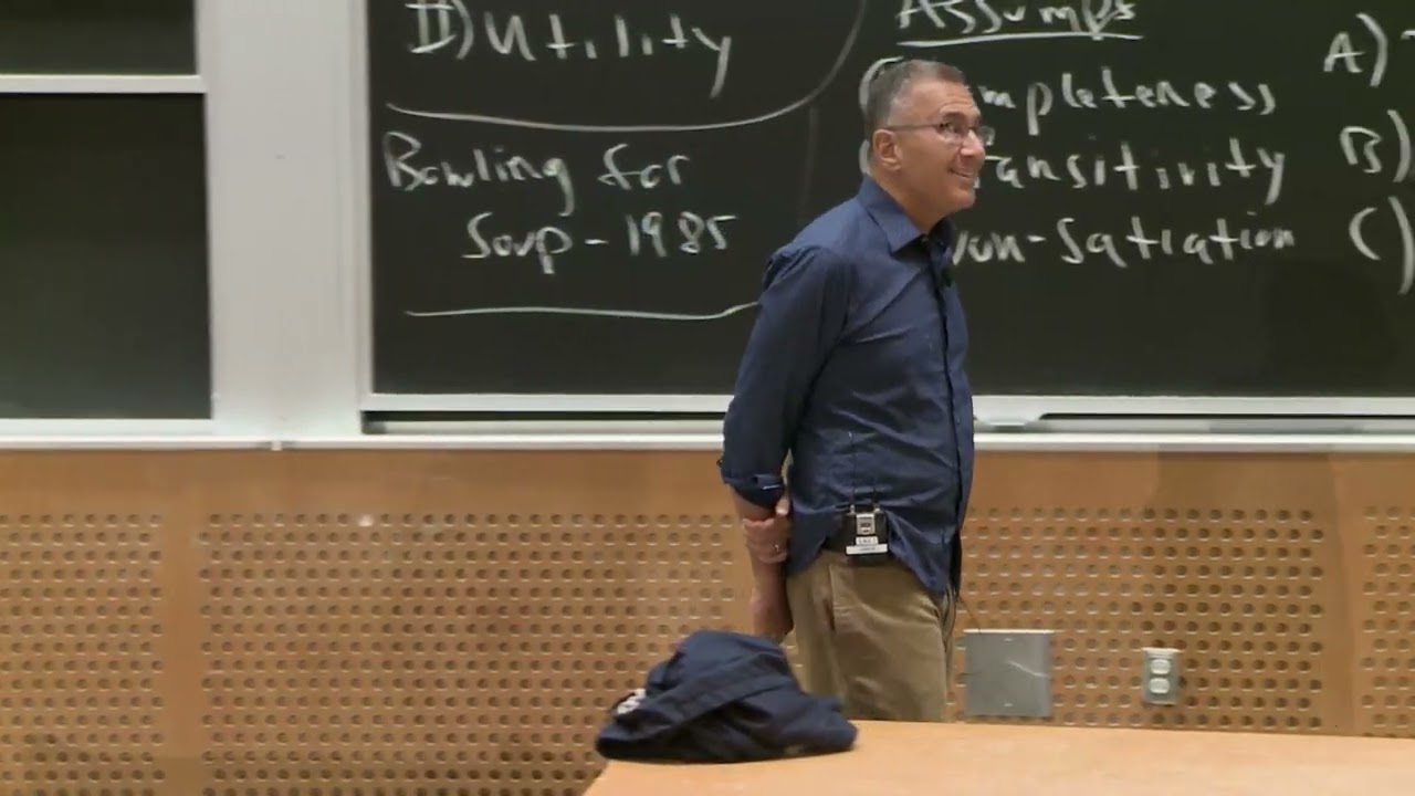
Lec 2: Preferences and Utility Function transcript
MIT OpenCourseWare · @mitocw
Words
6,872
Runtime
40:48
Speaking pace
168wpm
Reading time
29min
168 words per minute, between the 160 25th percentile and the 181 median of 349 measured videos. That distribution comes from the 349-video hook study.
Opening (first 30 seconds)
[SQUEAKING] [RUSTLING] [CLICKING] PROFESSOR: So today we are going to talk about where consumer decisions come from. Remember last lecture we built a supply curve and demand curve, and I just sort of made them up. And I said, now we're going to start to go back and build up where they come from. And today we'll start with the demand curve, and start by talking about consumer preferences. OK. So the first thing we're going to do is we're going to understand how
84 words, the words spoken in the first 30 seconds at 168 words per minute.
Sentence shape
| Measure | This transcript |
|---|---|
| Sentences | 679 |
| Average words per sentence | 10.1 |
| Longest sentence | 61 words |
| Questions asked | 55 |
| Sentences containing a number | 53 |
Most used terms
- ok107
- utility71
- pizza66
- indifference62
- cookies50
- marginal42
- preferences39
- curve37
- basically30
- indifference curve30
- point30
- slices30
Filler phrases
70 in total: basically 30 · like 22 · actually 5 · I mean 4 · right? 3 · kind of 2 · sort of 2 · literally 1 · you know 1.
A literal whole-word count of the same phrase list the Prepublish browser extension uses, so a phrase inside another word is not counted and a phrase used in its ordinary sense still is. It is a count and not a judgement.
What this transcript is
Every word below is the caption track YouTube publishes for this video, pulled from the video itself and reproduced unchanged. It is not Prepublish's writing, not a summary, and not a re-transcription: it is the video's own published captions. English captions, published by the channel, in the video’s original language. Source: the video on YouTube. A channel that would rather this page did not exist can ask for its removal through the contact page, and it is removed.
Transcript
[SQUEAKING] [RUSTLING] [CLICKING] PROFESSOR: So today we are going to talk about where consumer decisions come from. Remember last lecture we built a supply curve and demand curve, and I just sort of made them up. And I said, now we're going to start to go back and build up where they come from. And today we'll start with the demand curve, and start by talking about consumer preferences. OK. So the first thing we're going to do is we're going to understand how consumers make choices.
Now essentially as I mentioned last time, consumers make constrained choices. They essentially make themselves as well off as possible, subject to a limited budget. What we're going to start with today is forget the limited budget. Imagine we just all won the Mega Millions. OK. There's no budget. We're just going to ask, what do consumers want and not worry about how they're going to pay for it. OK. So today we're going to talk about preferences.
We're going to talk about what consumers want and how we translate those wants and desires into a mathematical formulation that allows us to derive demand curves. OK. So basically we're going to do this-- we're going to ultimately, for consumer demand, proceed in three steps. The first step is we're going to write down our underlying assumptions about consumer preferences. We're going to talk about how consumers-- talk about a set of axioms that determine the rules of consumer preferences across goods.
We'll then translate those set of axioms to a mathematical function we call the utility function, which is a mathematical expression of consumer preferences. And then next time, we'll introduce the budget constraint and talk about how consumers make choices given this mathematical utility function and given the budget constraint they face. OK. So that's the roadmap of where we're going. OK. So today we're going to talk about preferences, axiomatic rules of preferences, and how they translate into the mathematical rules that govern individual decisions.
So to do this, let's start by talking about preferences. And let's talk about the key assumptions we are going to make in modeling consumer preferences. So remember, all models make simplifying assumptions. We're going to make-- all inexact models make simplifying assumptions. We're going to make three assumptions here. The first assumption we're going to make-- so what are the key assumptions? The first assumption we're going to make is completeness.
That is, we are going to assume that when consumers are faced with two choices, they're either going to prefer one or prefer the other or be indifferent, but they're going to have an opinion. They're not going to say, I don't know. OK. Consumers will have opinions over all possible choices. They'll like one better than another, or they'll be indifferent, but they'll have opinions over all possible choices. It's a complete set of preferences.
The second thing is the same assumption we're making since kindergarten in all our math classes, which is transitivity, OK, which is the classic, if you prefer A to B and B to C, you must for A to C. I'm pretty sure all MIT students know transitivity by now. OK. So that is the second key assumption, which is, once again, not a big deal. The third assumption's where economics gets its power. The third assumption is a new one, which we call the assumption of non-satiation-- or new to you-- the assumption of non-satiation or basically, more is always better.
OK. So these assumptions are standard assumptions you make math class, complete choice sets, transitivity. Non-satiation is new to you. That's the assumption that basically more is always better. Now it doesn't mean more makes you equally happy. It doesn't mean the 10th thing makes you as happy as the 9th thing. It just means the 10th thing is always better than not having it. More is always better. OK. So basically, if you're offered something for free, you'll always take it.
OK. It's always better than not having it. That's because we live in a world of goods. Now you might be thinking to yourself, well if someone offered me for free to stick me in the eye with a needle, I wouldn't take that. And you're right, because that's a bad, for most people, I guess. But we're going to operate in the world of goods. So as long as things are goods, we always want more. Now, with those in mind, we can develop what we call indifference curves, which are essentially preference maps.
We're going to map people's preferences into a set of what we call indifference curves. So to do this, let's start with a simple example. OK. Imagine it's the beginning of semester and your parents are going to give you some money to buy the two things you care about, a slice of pizza and cookies. That's all you care about in this world. Once again, as someone asked last time, we're working with simplifying two-dimensional assumptions.
In reality, of course, you care about buying 20 different things, but the underlying logic won't change. The math will just get harder, and the graphs will become multi-dimensional and hard to see. So we're going to start with two goods, but everything we do here works with three, four, five, six, et cetera goods, OK, just harder math and graphics. So let's say I have two goods, and let's say you're going to face three choices.
Choice A is you can have two slices of pizza and one cookie. Choice B is you can have two cookies-- you can have, I'm sorry, one slice of pizza and two cookies. Or choice C is you can have two slices of pizza and two cookies. Those are your three choices you're facing. OK. And let's assume, given my preferences, that I'm indifferent between A and B. Let's assume that given my preference I'm indifferent between those two.
Now where does that come from? Well, we're going to take preferences as primitive. We're not going to question where preferences come from. People are going to have their preferences. It's genetics or nature or nurture or whatever. That's something we deep delve more deeply into when we think about deeper economics. But for now, for this class, we're going to do preference is given. So I have a set of preferences such that I'm indifferent between those two choices, but I prefer option C to both.
OK. I'm indifferent between A and B but I prefer C. OK. So we can now graph my preferences. Andrew, can I get a copy of the handout? So we can now graph my preferences. And the graph of my preferences is shown in figure 2-1. OK. Everyone should have a handout. Remember, they'll always be in the back when you come in. Please make sure you grab them as you come in. Figure 2.1 is a map of my preferences. OK, on the x-axis, OK, is, I believe-- let me just-- I'm going to look at yours for a second.
You can look at your neighbors. On the x-axis is cookies. On the y-axis is slices of pizza. OK. So different maps are essentially maps of how you choose between two goods you're choosing from. OK. So basically this is your indifference map. Thank you. This is your indifference map. And what you see is we have mapped the three points A, B, and C. A is two slices of pizza and one cookie. B is two cookies and one slice of pizza.
C is two of both. And we have drawn a curve between A and B. We label this an indifference curve. It's an indifference curve because I said you're indifferent between A and B So one indifference curve goes through both A and B because you're indifferent between those choices. Remember, completeness says you can't not care. Completeness says you have to choose. But it's OK to be indifferent. OK. But point C is on a higher indifference curve, because you prefer point C to both.
OK. So there's going to be four properties of indifference curves. These are indifference curves, which you're going to work with extensively throughout the semester, are going to have four properties. Properties of indifference curves-- the first property, OK, is, consumers prefer higher indifference curves. So the further out the indifference curve is, the more preferred it is. OK. And that just follows from non-satiation.
More is better, so quantities that are further out away from the origin are better. OK. The second property is indifference curves are downward sloping. We're not saying anything about the shape yet, just the slope, that indifference curves are downward sloping. And once again, this follows from non-satiation. Why? Because if indifference curves were upward sloping, you wouldn't satisfy non-satiation. Look at figure 2-2 with an upward sloping indifference curve.
This is just one particular kind of upward sloping indifference curve, but it's true for all of them. If the indifference curve is upward sloping, that means you'd be indifferent between one cookie and one slice of pizza and two cookies and two slices of pizza. That would violate non-satiation. You can't be indifferent between less and more. You have to always like more better. So indifference curves have to be downward sloping through non-satiation.
OK. The third is, indifference curves never cross. Indifference curves never cross. And the reason indifference curves can't cross is because that would violate transitivity, and more is better. So let's look at figure 2-3 with crossing indifference curves. OK. In this graph, figure 2-3, A and B are on the same indifference curve, and A and C are on the same indifference curve. That means you must be indifferent between A and B and indifference between A and C.
Well if you're indifferent between A and B and B and C by transitivity, you must be indifferent between B and C. But that can't be true. You can't be different from B and C because B is more than C. OK? B is a dominant-- you get the same amount of cookies and more pizza. So you, by definition, have to like B better than C. So you can't be-- it violates jointly transitivity and non-satiation. OK. So that's the third property.
And the fourth property is basically completeness, which we express as, only one indifference curve through any given point. You can't have two indifference curves that cross through one point. OK. So one 1 IC through any given point per point. Per precise allocation it will be 1, because otherwise you wouldn't know how to feel. OK. There has to be one indifference curve for every precise point. OK. So with these rules in mind, let's talk about how you can use indifference curves.
Here's how I learned about indifference curves. When I was a student in 1401, here's how I learned indifference curves. Actually it was a semester later. I still didn't quite understand when I left 1401, because I wasn't as smart as you all. OK. But I had a year off, and my year off was with a graduate student. And this graduate student was trying to decide on where to go for their job. And they said to me, look, we can express an indifference curve.
This is one of the few graphs I'll draw for you this semester. He said, look, there's two things I care about. I care about school quality, like how highly ranked is where I'm going to go, are my colleagues the smartest, et cetera, and I care about location, which is, how's the weather? Will, this is weather. OK. And he had two choices. His choices were Princeton, great quality, mediocre weather, or Santa Cruz, not as good quality, great weather.
If you've ever been to Santa Cruz, I don't know how anybody studies there. You can walk out, steps out and surf. OK. And he basically said, look, at this point I'm indifferent. I'm indifferent between better job at Princeton, but mediocre weather, and a worse job at Santa Cruz-- no offense to Santa Cruz. Princeton's an amazing place. Santa Cruz is still a great place, but it's not Princeton. OK. A worse job at Santa Cruz and awesome weather and being able to surf every day.
So he said, I'm indifferent. He said, in the end, what did he decide to do? In the end he decided to go to a place called the IMF, which is not the thing from the Tom Cruise movies, but actually the International Monetary Fund, because that was in DC, which had better weather. So it wasn't as good a job as Princeton-- this is Princeton, this is Santa Cruz-- but it was better weather. It wasn't as good weather as Santa Cruz, but it was a better job.
And he decided that combination made him happier. Is he right? No, he's not right. There's no sense of right. Preferences are your preferences. OK. You might all feel very differently about this set of choices. This isn't when everybody's preferences are correct or wrong. OK. This is just how we thought about this job choice and how we used an indifference map to explain it. OK. Questions about that? Questions about how these indifference curves work?
Yeah. AUDIENCE: [INAUDIBLE] PROFESSOR: Speak loudly so everyone can hear. Thanks. AUDIENCE: What would an indifference curve where you prioritize quality a little bit more? PROFESSOR: That's a great question. So basically, once again, the question is, how do you put quality into this framework? Well, essentially what you would do is you would say then I have two dimensions. It's be quality and quantity of one good. You'd have to add either a third dimension or you'd say it's a different choice.
So what we'll do a lot in this course-- you can think of sequential choices. So let's say, for example, you want to decide between cookies and pizza. You decide. And now within cookies, if you decide, I want to allocate $6 to cookies, now you say my choice is one unbelievable $6 cookie or six terrible $1 cookies. That's a new indifference curve. You've already decided first how many you're going to spend on cookies. So we can always break any monster decision to a set of sequential, two dimensional decisions.
So that's how you do it. OK. Good question. Other questions. Yeah. AUDIENCE: So, like, for number [INAUDIBLE]. PROFESSOR: Yeah. AUDIENCE: One curve per point. That's like saying that, like, they're never crossing. PROFESSOR: Yeah. I always get that question. It's technically different, but effectively the same. OK. Good. If I don't see your hand, by the way, shout out. It's a big classroom. OK. So now we're going to move on from preferences and go on to talking about utility.
OK. Point two, topic two, utility. OK. So basically, underlying where preferences come from is a mathematical function we call the utility function. It's basically how we mathematically represent these graphical indifference curves. OK. So, of example, a common form of utility function we'll use a lot this semester is the log utility function, which we express the form, utility is the square root, in this case of pizza slices times the number of cookies.
That is a mathematical representation of preferences. It says my utility is a square root of the number of slice of pizza times the number of cookies. S stands for pizza because it slices, because we use P elsewhere for prices. I don't want to be confusing. OK. So that says-- note this is consistent with what I wrote up there about indifference curves. Two slices of pizza and one cookie gives me the square root of 2 utility.
One slice of pizza and two cookies gives me the square root of 2 utility. So I'm indifferent. Two slices of pizza and two cookies gives me 2 utility, so I'm happier. So this is consistent with the indifference curves. Yeah. AUDIENCE: What is [INAUDIBLE]? PROFESSOR: That's a different indifferent. You could write down-- like I said, I'm not judging anybody's preferences, but that would be a different mathematical function.
This is one of an infinite set of mathematical functions to write down. This is not a true representation. This is an example. You can write any utility function you guys want to think of. We can write it down and we'll write down many of them this semester. But I need to work with this one first until we understand the rules. Yeah. AUDIENCE: [INAUDIBLE] So why do you [INAUDIBLE] decipher [INAUDIBLE]. PROFESSOR: Well, no.
But it shows your indifferent between S And C. But it would show that you prefer more of both. But it's true. It shows you're indifferent between S times C. That's absolutely right. AUDIENCE: I think [INAUDIBLE]. PROFESSOR: Between what? AUDIENCE: Like [INAUDIBLE]. PROFESSOR: Same as what? AUDIENCE: Because if we said, like, [INAUDIBLE] equals a constant for both types of functions and the-- AUDIENCE: Like why do we need square root [INAUDIBLE]?
AUDIENCE: Yeah. PROFESSOR: Oh, that's a great point. That's an excellent point. The reason we're going to need square root is because it's a form of preferences-- it's a rule on preference that going to help us do a lot of things well in this semester. I'll explain that in one minute. It's a good question. Now I understand. Thank you. Yes. In fact, that question leads to a natural next question, which is what the hell is utility?
What does it mean? And the answer is, utility means nothing cardinally. It only has meanings ordinally. That's what I mean is a utility of 3 is a meaningless concept. Utility only matters in an ordinal sense, in the sense of ranking choices. So utility functions will simply be mappings that we use to rank choices, not mappings that we use to say this choice is 50% better than that choice. It's only for ranking. So the number itself doesn't matter.
And by that same question, well, the ranking of S times C is the same as the ranking of squared S times C, so why do we write it that way? OK. And the reason we write it that way is because utility functions of this general form, of this power form with less than 1, will deliver an important real world consequence. And we see that through the notion of marginal utility. OK. So once again, this is just one form of preferences.
The question is absolutely right. This mapping would work just fine as S times C or S-squared times C-squared or S to the millionth times C to the millionth. Because the numbers don't matter. It's the ranking that matters. All those are the same ranking. But those functions deliver something very different, which would violate the way we think about the real world, which is that basically the fundamental driver of all consumer decisions we'll make this semester-- remember I said, I'm going to tell you 100 times things are really important.
This is really important. OK. The fundamental driver is the key assumption that we make of diminishing marginal utility. That is, we assume more is better, but the next unit is not quite as good as the one before. We assume marginal utility diminishes. We assume each additional unit makes you less happy than the one before, which wouldn't be true if we didn't have the square root function there. OK. Why do we assume that?
Because it makes sense. OK. It makes sense that basically the 10th slice of pizza makes you less happy than the ninth slice of pizza. It makes sense that the fifth cookie makes you less happy than the fourth cookie. It makes sense that your fifth favorite movie makes you less happy than your fourth favorite movie. Now, it could be tiny increments between them, but it makes sense that when you rank things, the next one is worth less.
OK. So, for example, let's go to figure 2-4, and let's hold the number of pizza slices-- by the way Andrew, we should change that to, instead of holding pizza, we should say hold pizza slices. OK. Let's change the number of pizza slices constant at 2. Let's assume you for sure decide you want two slices of pizza. Now you're going to ask yourself, how does my utility vary as I have additional cookies? The answer is, if I have one cookie, my utility is 1.4 square root of 2.
If I have two cookies, my utility's 2. If I have three cookies, it's 2.45 and so on. OK. Basically what you see is that the incremental utility from each additional cookie is falling. That's shown in figure 2-5. Figure 2-5 illustrates diminishing marginal utility. Each additional cookie makes you less happy, holding constant the number of pizzas. OK. So basically this is an enormously sensible assumption. It's an assumption.
As I said, no one can tell you what your preferences should be. But it turns out, we think most people's preferences satisfy the principle of diminishing marginal utility. And that is going to drive a lot of the mathematics we're going to do this semester. We will give you examples where it's not true. We'll give you examples of increasing marginal utility and constant marginal utility and have you discuss them. But we're going to generally assume diminishing.
Question. AUDIENCE: [INAUDIBLE]. Doesn't it-- does it violate nonsatiation because it implies that you have no pizza but you have cookies? Then there's no utility? PROFESSOR: That's a great question. That's essentially, with these preferences, it would say that essentially your preferences are such that if you can't have a cookie, you don't care how much pizza you get. That doesn't violate nonsatiation because basically that is-- nonsatiation says more of everything is better.
It doesn't say more of one thing is better, more of any one thing is better. Nonsatiation says more of everything is better. It can't be true that if you get more of everything, you're better off. It can be true, getting more of one thing doesn't make you better off. So think about left shoes and right shoes. OK. It doesn't matter how many-- if you only have one left shoe, it doesn't matter how many right shoes you have.
So it doesn't violate more is better but you'd be better off with two left shoes and two right shoes than one left shoe and one right shoe. Yeah. Good question. Good. I love these questions. Thank you so much. OK. So basically, with that in mind, let's talk about, how do we-- we can now go back and ask, well what drives the shape and slope of indifference curves? OK. So what is the slope of the indifference curve? The slope of the indifference curve is the rate at which we're willing to trade off-- just definitionally, mathematically-- the rate at which we're willing to trade off slices of pizza for cookies.
OK. The rate at which we're willing to trade off, basically one good for another. OK. So we'll call that delta-S, delta-C is the slope-- at any point that's the slope of the indifference curve. The rate at which you're willing to trade the good on the y-axis for the good on the x-axis. We're going to just define it this way for convenience. Obviously you can invert it. It doesn't change anything. But for convenience we'll always think of it this way.
The rate at which you're willing to trade the good on the y-axis for the good on the x-axis. OK. And we're going to call this the marginal rate of substitution. The MRS, a key concept for this class, the MRS, the marginal rate of substitution. OK. That is the rate at which you're willing to trade off the good on the y-axis for the good on the x-axis. OK. Now, you're not really trading. We're not in some ancient barter system where you're trading pizza for cookies.
But effectively you are because of opportunity cost. Given a budget-- we haven't given you a budget yet, but next time we will-- given a budget, any money you spend on pizza you can't spend on cookies and vice versa. So effectively it's a trade. By buying a slice of pizza, you're essentially trading away cookies. Not that you're trading them away but you're trading away the money you could use to buy cookies. OK. So in a world with only two goods, whenever you buy one, you're trading away the other.
Now that doesn't operate directly. It operates through the budget constraint. But that's the way to think about it. So you're substituting pizza for cookies. Now how does this relate to the utility function? Well here's what's kind of cool. OK. Think about an incremental move along an indifference curve. An incremental move along an indifference curve is essentially, you're giving up a little slice of pizza to get a little more cookie on the margin.
So that's saying, you give up delta-S times the marginal utility of slice. So you give up a little bit of slice of pizza, which you liked MUs, that's your marginal utility for pizza, and you're getting a little more cookie, which you value at your marginal utility for cookies. OK. That's the equation of-- that's a delta along that curve. OK. You give up a little pizza, which costs you your marginal utility of pizza. You get some cookies, which gains you marginal utility of cookies.
OK. Rewriting this, we get that delta-S delta-C, which I said is the MRS, is equal to minus MUc over MUs The MRS is the ratio of marginal utilities. That is, the slope of the indifference curve is the ratio of the marginal utilities. And that's how we tie the math and the graph together. That's how we bring the math and the graph together, that basically the slope of the indifference curve is the MRS is the negative opposite of the ratio of marginal utilities.
Now this is very tricky. Here's the one thing you need to keep in mind, which is to remember that the reason there's a negative sign is that marginal utilities are negative functions of quantity. The more you get, the lower your marginal utility is. Utility is a positive function of quantity. But because of diminishing marginal utility, marginal utility is a negative function of quantity. You got to embed that in your brain.
OK. More is better says utility is a positive function of quantity, except of course in this important case that was pointed out there, positive function of both things going on. But marginal utility is a negative function of quantity. OK. You're less happy by the next incremental unit than you were by the ones before. OK. So basically, as you get fewer slices and more cookies, what is happening? Well, the marginal utility of slices is rising.
You're giving up pizza slices so your marginal utility's going up. The marginal utility of cookies is falling. OK. So what you get is basically a decline in the value of the MRS. The margin utility of pizzas is slightly rising. OK. Margin utility of cookies is slightly falling. This ratio falls, so the MRS falls, so you get this downward sloping indifference curve. OK. So this is sort of hard. So let's see this mathematically and graphically.
Let's start with the math. OK. Let's start with the math. OK. We said utility is the square root of S times C. OK. So what is the marginal utility of cookies? We're just going to differentiate this with respect to C. Differentiate this function with respect to C, what do you get? So delta-U, delta-C you get 0.5 times the number of slices of pizza over the square root of S times C. OK. What is the marginal utility of pizza, slice of pizza?
You get DU DS equals 0.5 times C over square root of S times C. And once again, I apologize for the handwriting. Please ask if it's not clear. OK? So I'm just differentiating this function to get the two marginal utilities. OK. If I take, based on these two marginal utilities, the MRS, which is the negative of the ratio, the MRS equals minus S over C, for this particular example. These aren't general rules I'm deriving here.
For this example the MRS is minus S over C. So basically, what the MRS is showing you is that the MRS for slice of cookies-- for slice of pizza opposed to cookies is rising as you get more slices and falling as you get more cookies. So let's see this in figure 2-6. OK. Figure 2-6 shows the indifference curve again, but now with the MRS is plotted. Remember, the indifference curve is not linear in this case, so the MRS changes along the indifference curve.
So I'm giving you local approximations to the MRS at different points in the indifference curve. But it's very important to remember-- this is key-- because the diminishing utility, you are going to get-- yeah. AUDIENCE: So, like, in this formula, like the marginal utility is given that by differentiating [INAUDIBLE]. Right? PROFESSOR: Right. AUDIENCE: But in figure 2.5 by [INAUDIBLE]. PROFESSOR: Yeah. Yes. Figure 2.5 is just giving you local approximations.
Those points are solved by differentiation, but those are local approximations. OK. Yep. So basically, that's the thing. Our graphs are never going to be as precise as our math, because we essentially want to use linear mathematics fo for nonlinear graphs, and so we're going to end up with a lot of local approximations. OK. So basically, in other words, at point A, OK, at point A you have four slice of pizza in one cookies.
At point B You have two of each. And at point C you have four cookies and one slice of pizza. And according to this utility function, you're indifferent. Right? All those give 2 as the utility. All those combinations give you a utility of 2. You're indifferent. OK. But at point A, even though you're indifferent between all three points, they have very different MRS'. At point A, the MRS is minus 4. You would be willing to give up four slices of pizza to get one cookie.
At point C, the MRS is minus 1/4. You'd be willing to give up only one slice of pizza to get four cookies. Why? What's changed between points A and C? Why has the MRS changed so radically between points A and C? Yeah. AUDIENCE: [INAUDIBLE] PROFESSOR: What? I'm sorry? AUDIENCE: You have less slices of pizza. PROFESSOR: You have fewer slices of pizza. Exactly. So, basically, what's happening is, as your slices of pizza falls, and then by definition your cookies goes up, your marginal utility of pizza rises, and your marginal utility of cookies fall.
When you're at point A, you really want pizza. You're happy to give cookies to get pizza. I'm sorry, you really want cookies. I'm sorry. My bad. At point A, you really want cookies. You got four slices of pizza. You're full already. You want a cookie. OK. When you're at point C, it's like, what are you going to do with four cookies? You're not going to have enough protein in your dinner. Your mom will be upset. OK. So you basically want to trade some of those cookies back for some pizza.
OK. And then at point B, you see the MRS is minus 1, because given this utility function, at that point you're essentially indifferent. You're indifferent between pizza and cookies at point B. OK. So that is why we graph the indifference curves in this way as concave indifference curves, concave to the origin, because basically we want to satisfy this principle of diminishing marginal rate of substitution. For those who really want to be technical, the real technical definition is diminishing marginal rate of substitution.
You don't always have to have diminishing utility. We generally do. You can write down functions which don't have diminishing utility but do have diminishing marginal rate of substitution if you are so inclined. The technical definition is that what drives utility theory is diminishing marginal rates of substitution. But almost always we'll have diminishing marginal utility as well. That's all I'll say about it. You can forget it if you want, but if it's bugging you, that's why.
OK? Now, consider what it would be like-- I'm sorry. So it's convex to the origin. My bad, I'm sorry. Convex to the origin indifference curves. Convex indifference curves. Consider what it would be like with a concave to the origin indifference curve, as in figure 2-7. Consider what life would be like. We often do proofs by the negative. OK. This is for the utility function. Figure 2-7 is drawn for the utility function, x-squared plus y-squared equals 65.
That's the utility function of this graph there. Well, I shouldn't say S-squared plus-- I shouldn't say x and y. I should say S-squared. S-squared plus C-squared equals 65. OK. Now once again, you can't tell me that utility function is wrong. People have different preferences. But it doesn't satisfy what we would think is a common sense principle, which is that would say that when you have eight slices of pizza and one cookie, you'd be willing to give up-- when you have eight slices of pizza and one cookie, you would give up only an 1/8 of a slice of pizza to get a cookie.
So you really wouldn't give up much pizza to get a cookie. And yet, when you're down all the way of having seven cookies and four slices of pizza, then you give up almost two slices of pizza to have a cookie. It doesn't make sense. Why would you give up more pizza when you have less pizza? When you already have eight slices of pizza, why are you less willing to give a pizza for a cookie than when you have more slice of pizza-- when you have fewer slices of pizza and more cookies?
It doesn't make sense. Now, it doesn't make sense-- let's be clear. I'm not saying it is inconsistent with reality. OK. Like I said, we don't have strict laws like E equals MC-squared in this class. There's someone out there who has these preferences. I guarantee it. What I'm saying is, most people do not. And so we're going to try to, in this class like I said, make a series of simplifying assumptions that explain most of reality, even though it doesn't explain 100% of reality.
OK. And diminishing MRS is one of those assumptions OK. And that's why diminishing MRS makes sense because it delivers the fact that the more you have of one good, the less you care about having the next unit of it. OK. Let me stop there. Questions about that? This is really, really important to all of consumer theory. It's actually going to be important for production theory to this general notion of diminishing-- production, we're going to call it diminishing marginal product.
But it's going to be the same of thing. So questions about where this all comes from. OK. You know, throughout this class, you want to ask yourself, does this pass the mom test? That is, could you go home and explain this to your non-economist mom? And you should understand this well enough that you can. OK. I don't know if she'd be interested. But it doesn't matter. She's your mom. She has to listen to you. So basically, make sure you understand it that well.
OK. Now, let's go to an example. Yeah. Sorry Go ahead. AUDIENCE: What's the point of a concave indifference curve then? PROFESSOR: The only point of a concave curve would to represent the set of preferences I wrote there. I mean, there's no point or not point. It's just simply saying that there exists someone in the world who has that utility function and this is their preferences. But you won't generally ever see one.
Does that make sense? AUDIENCE: Yeah. PROFESSOR: All right. OK. So let's go to an example. There's actually a wonderful example of diminishing marginal utility and how it operates in the real world, which is different sizes of consumer goods of consumer consumption goods. So, for example, at Starbucks, according to Alex's detailed research, you can get a tall iced coffee for $4.55 or you can get twice as much coffee, whatever the hell they call the big one, for 90 more cents.
So $4.55 for the smallest, 90 cents more to double your amount of coffee. Or McDonald's. A small Coke is $2.29. A large Coke, which is more than twice as big, is $2.99. So essentially you are paying much less to increase the quantity. Why is that? Yeah. Loudly speaking here. Go ahead. AUDIENCE: Because you get less marginal utility as you're getting the next unit of drink. PROFESSOR: Exactly. So you think about yourself walking to McDonald's on a hot day, OK, or Starbucks on a cold day and you really need to be sated.
You're either very, very cold or very hot. You need to be sated. But a small will get you most of the way there. Now a large is better. Buy more is better, but it's not as much better. You just need it to be sated. You need to make sure you got your liquids in. So you are not willing to pay as much for the incremental quantity. You're not willing to pay as much. And the key thing is basically that companies recognize this.
And this is where we start to dip into producer theory. Companies are making their business decisions based on what they know about consumer preferences. This is why someone asks, why do we ever have a concave indifference curve? This is why companies don't believe there are concave indifference curves, because they price this way. They know that most people care less about the additional 16 ounces than they do about the first 16 ounces.
Now if maybe you all thought that was common sense, or maybe you never thought about why that is. But this is, once again, an illustration of how a common phenomenon in society that exists everywhere can be explained by what's an incredibly simple model. Remember, we came into this class knowing nothing about utility and all that stuff. I've already gone on and explained an incredibly important phenomenon in the world.
And there's many other choices and things that you'll see that can be explained by this model. OK. Questions about that. Yeah. AUDIENCE: So how does that benefit Starbucks or McDonald's, because it still costs them the same amount to produce? PROFESSOR: Great question. Someone want to answer that? How does it benefit Starbucks and McDonald's? Yeah. AUDIENCE: If they price it more, no one's going to buy the larger sizes.
PROFESSOR: Yeah. So basically, essentially the calculation-- we aren't going to produce a theory yet, but I'll give you a heads up. The calculation of McDonald's and Starbucks are doing are, I want to-- you're right. I mean, the cost the inputs of this stuff are so cheap. I mean, you'd be disgusted how-- McDonald's, for their sodas, it's like probably about three to four cents for them to make a soda, in terms of the marginal cost of a soda.
OK. So let's say it's $0.03 for a small and $0.04 for a large. OK. So basically, if preferences were such-- and you could write preference this way, where I never want anything more than a small. Like literally our stomachs can't hold more than a small, then nobody would pay a penny more for a large and they wouldn't make it. But nobody's that way. Most people pay a penny more for a large. So then your question is, how much more can I charge before people don't want the larges anymore?
And that's essentially the calculation they're doing. They've computed-- and they've got people, hundreds of people doing this all the time saying, look, if we charge $0.69, people buy the large. If we charge $0.70, people buy a couple fewer larges, but we make $0.01 more. But once we go above $0.71 it no longer makes sense. And that's essentially the business decision-making we'll talk about in a few lectures, which is, how do businesses decide how to set their prices?
Here we're just showing they set their prices in response to a principle we now know is generally true, which is diminishing marginal rate of substitution. Other questions? Good question. Other questions. All right. Well let's stop there. It's a little early, but that's all I got for today. So we will come back on Wednesday and we'll talk about what happens when you actually have a limit on how much you can spend.
The words are the caption track's own and nothing is reworded or re-transcribed. Paragraph breaks are placed between sentences so the text reads as prose.
Use this transcript
Three free tools that work on the material around a video like this one. No signup, no login.
Hook Analyzer
Paste the first 30 seconds of your own draft for a hook score and rewrites.
Policy Pre-Flight
Check your draft against YouTube's advertiser-friendly guidelines before you record it.
Channel Skill Generator
Read this channel's public videos and transcripts, and download a writing brief for it.