Getting the transcript
Reading the captions from YouTube. A video nobody has opened here before takes 10 to 30 seconds; this page fills in on its own.
Getting the transcript
Reading the captions from YouTube. A video nobody has opened here before takes 10 to 30 seconds; this page fills in on its own.
Quantopian · @Quantopianvideos
Where viewers went back to watch this video again, from YouTube's public Most replayed graph, lined up with what was said at that moment.
Most replayed moment #1
2:392.6x the video's typical replay level
latch or latex or however you'd like to pronounce it um latch math formulas you can put those in so here I'll put in a Lotte math formula and I'll put in a display mode formula and we'll say 2x^
Said at 2:31
Most replayed moment #2
20:132.6x the video's typical replay level
trading days remember we don't trade every day so 857 trading days worth of data and six columns and those columns include price H low uh you know volume all these other fields that people generally use you can also get a minutely frequency data uh I'll leave
Said at 20:06
Most replayed moment #3
22:132.0x the video's typical replay level
price on the Y AIS which is already pretty useful so there's Microsoft over these three years and now let's actually get the mean and standard deviation for Microsoft and there you go the next thing we're going to do is we're going to look at how to get returns from
Said at 22:07
The graph counts replays. It does not show where viewers stopped watching.
Words
5,922
Runtime
33:09
Speaking pace
179wpm
Reading time
25min
179 words per minute, just under the 181 median of 349 measured videos. That distribution comes from the 349-video hook study.
Opening (first 30 seconds)
all right hello everybody this is um the video recording for the introduction to research lecture in the quantopian lecture series and as always with these videos I am going to show you how to get to the lecture Series so uh one of the ways is to type www. quantopian we're going to be talking about today is number one introduction to research so research is the research environment in quantopian and I'll show you what that means if you haven't seen the research environment before uh it is
90 words, the words spoken in the first 30 seconds at 179 words per minute.
Free, no signup. See how the first 30 seconds hold attention, with rewrites.
Sentence shape
| Measure | This transcript |
|---|---|
| Sentences | 11 |
| Average words per sentence | 538.4 |
| Longest sentence | 1,672 words |
| Questions asked | 0 |
| Sentences containing a number | 6 |
Most used terms
Filler phrases
178 in total: uh 87 · um 39 · like 22 · you know 16 · kind of 6 · actually 5 · basically 2 · I mean 1.
A literal whole-word count of the same phrase list the Prepublish browser extension uses, so a phrase inside another word is not counted and a phrase used in its ordinary sense still is. It is a count and not a judgement.
Free, no account. See where attention is likely to drop, with a rewrite for each weak line. The free check shows the scores and the one issue costing the most. Or run it on the words above first.
Free · No login · See a sample audit first if you prefer.
What this transcript is
Every word below is the caption track YouTube publishes for this video, pulled from the video itself and reproduced unchanged. It is not Prepublish's writing, not a summary, and not a re-transcription: it is the video's own published captions. English captions, generated automatically by YouTube, in the video’s original language. Source: the video on YouTube. A channel that would rather this page did not exist can ask for its removal through the contact page, and it is removed.
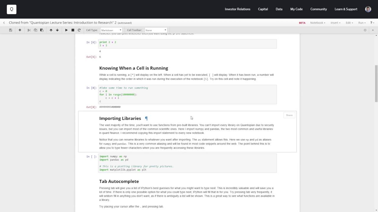
all right hello everybody this is um the video recording for the introduction to research lecture in the quantopian lecture series and as always with these videos I am going to show you how to get to the lecture Series so uh one of the ways is to type www. quantopian we're going to be talking about today is number one introduction to research so research is the research environment in quantopian and I'll show you what that means if you haven't seen the research environment before uh it is based on the IPython notebook uh now known as the Jupiter notebook and IPython notebooks are combinations of code cells and text cells which is really powerful so for example um here I have a text cell and if I double click on this cell you can see well it's just text with a little bit of formatting so you can see these hashtags make uh titles and um if you execute a cell using the play button right here I'll run it it'll render that cell and make the text nice and readable uh the other way you can execute a cell is by hitting shift enter just like that so I'm going to use shift enter a lot so if it looks like cells are executing by Magic uh that's probably me just hitting shift enter uh and I encourage you to learn that command too uh the other commands are up here on the control bar they should be pretty intuitive um save your notebook save it often uh make a new cell so when you make a new cell you can choose what type of cell it is with this drop- down menu so if it's a code cell uh you can see here I just have 2 + 2 um I'll replicate that in this cell so 2 + 2 and I execute that gives me four great uh but if I want to make it a text cell I switch to markdown don't worry too much about these other two types of cells for now I rarely use them the two important ones are code and markdown remember markdown is just the text formatting language so here's 2 plus2 and if I render that cell it's going to be rendered into text uh the other really nice thing is that you can have uh for those of you that are familiar with latch or latex or however you'd like to pronounce it um latch math formulas you can put those in so here I'll put in a Lotte math formula and I'll put in a display mode formula and we'll say 2x^ squared plus Z subt or something you know whatever you want to say so and you'll get this nicely rendered math it's really useful because what it allows you to do is it allows you to write out documentation for your analysis right next to your analysis and it's really taking off um notebooks of these form are taking off in research and in Industry um if you're familiar with ligo and the recent discovery of gravitational waves they released all of their analysis documentation and code to ReDiscover gravitational waves if you want to um in IPython notebooks and you can look it up if you look up ligo liigo I python notebooks they're really cool so these are useful because they're self-contained things if you send someone an IPython notebook they have the code to run some analysis and they have the documentation and the motivation for the analysis um it's really kind of a self-contained unit that allows researchers to work really effectively uh and so we'll show you some of the ways that you can do that here so again we've just been over executing a command and so now we're going to go ahead and execute this cell which you've already seen but we'll do it again 2+ 2 gives us four great so that's a code cell it evaluates what's in this cell now sometimes there is no result to be printed uh and you can see that as is the case with assignment so if we evaluate this cell we don't get anything now why is that well only the last line is printed in a Cell so in this case we'd print the last line but in this line the last line in the cell xal 2 doesn't return return anything so we have nothing to print so nothing is printed we'll see an example of this 2+ 2 3 + 3 you can see it prints out six and that's because 2 plus 2 is evaluated but we're not storing the results anywhere and we're not printing the results anywhere on the other hand the last line of the cell by default is evaluated that's 3 + 3 that returns six so we return six uh another important thing about notebooks is that memory space is uh basically kept between cells what do I mean by that well we set x equals 2 you'll see this a little more in the notebook I'm just going to stress it now we set x equals 2 so if we made a new cell and we said X we're going to get two so if you do something in one cell it affects all the other cells as well that's really useful but just remember that because it can also be a source of bugs right so if you make a list of cells that you evaluate in a certain order and then in your analysis you forget about one cell that like updates a variable that you need sometimes you'll accidentally run that cell and overwrite a variable that you needed or or whatever there's a lot of ways in which bugs can come out of this so just be aware remember that cells affect other cells all right so if you want to get it the result of something that's not in the last line well here's an easy way to do it you can just say to print that line and there we go so we have now 2 plus 2 is 4 3 + 3 is 6 here's another important thing about research you want to know when a cell is running well when a cell is running there's going to be a star on the left so um you can see here it has yet to be executed which means it's got this nothing displayed right here uh and then we'll run this cell you see the stars there and then after a little while uh it finishes and prints out uh whatever the sum is of that series that we made um and you know so we'll just do it one more time so you can see it's going to be a little fast there you go takes about one second to run um and uh while it's running you can see it has a star this is useful because sometimes you'll have slow commands uh you can know what cells are running in a notebook which haven't finished yet uh especially if you're running cells out of order in a more complicated analysis and as as always with these notebooks I strongly encourage enourage you to follow along with your own notebook while I'm doing this so if you want to go to the quantopian website uh get a copy of your lecture uh follow along if you have like uh the video running in one side and the lecture running on the other side maybe you have two screens that's I think the most powerful way to learn this um and then what you can do is you can pause the video and start messing around change this number uh change what's calculated here uh change these print statements you know as we get more complex there'll be more opportunities to mess around and try stuff on your own in my experience that's the really effective way to learn this stuff so here's the next subject importing libraries so the vast majority of the time you're going to need stuff that's you know not default in Python and so there's lots of pre-built libraries that have lots of useful functionality um for example numpy numeric python is a really important and common one in pandas uh this is a data processing Library uh actually written for p uh for finance it's really powerful we're not going to get to see too much of the power today because this is a really introductory lecture um but take my word that this is a really useful library that is going to save you a ton of time and then finally we have a plotting Library uh again don't worry too much about the syntax of this for now just kind of accept it say this okay this thing works we have it uh and then as you learn more about python if you don't already you'll you'll understand what's going on here um the important thing to noce that the as Imports stuff as another name so let's take see what that looks like so if we were to just import numpy we would have access to numpy and we would be able to say numpy uh and then we would say numpy do mean of a short array 1 2 three execute that cell and there's the mean too um but let's say that we wanted to call it something else we import numpy as cool uh stuff we could also do that and now we could just say cool stuff. mean so all it's doing is it's changing the name and you can see here we're importing these libraries as these shorter names so that we don't have to type out this long thing every time we want to do useful useful stuff so here now I can just do numpy mean of a short array um don't worry if you didn't understand that syntax yet you should hopefully understand it more and more as you go through these notebooks so the next really useful thing is tab autocomplete uh this is maybe the most useful thing in this notebook um tab autocomplete uh allows you to get access to stuff and see what's available in a library so you can see if I type a DOT and then tab it shows me all the suggestions and if I start typing out something like normal it will start Nar you can see I made a mistake there so it stopped narrowing it down because it didn't know what to do but if I start typing out normal it'll show me the options that are left or if without pressing tab I just type norm and then tab you see how it aut completed it I'll do it one more time if I type out nor or n o head tab there's the options that are left if I get to something where there's it's unambiguous it'll just finish the word for me so my recommendation is just to be constantly hitting tab as you're writing there's no loss if it's unambiguous it'll just finish your word for you and if it is ambiguous it'll show you some suggestions either way you're gaining information or getting something done faster so next question okay we've just found that there's this thing called uh numpy random. normal what does that even mean I like I don't what is that right so here's how we can check that getting documentation help this is a really important one if you put a question mark after an object in Python it'll return to you any documentation that python has about that object specifically for advanced users it's returning the doc string but we're not going to worry about that too much right now so let's execute this cell and there you go you can see it's returning this documentation of this function how do we use it what what does it do what are the arguments that we provide to it uh what are the outputs some references you can read up it's really useful it gives you pretty complete information and it pops up in this nice little popup uh so that you can kind of continue your work and maybe type some stuff up uh and and try using the function while reading the documentation so it's a really powerful tool tab complete and question mark notation I use all the time because I don't remember what everything does I just trust python to remember it for me and then I use the question mark to remember what stuff does so we're going to use that function now we're going to sample some random data so we're going to draw data from a normal distribution um and if you unfamiliar with sampling data there's some other lectures in the lecture series that discuss this specifically random variables um or you can look up on you know online what is sampling data but the general idea is that you have some distribution of possible data and you draw randomly from that distribution so a normal distribution is parameterized it says where is the center of the distribution so where is most data going to come from basically how wide is the distribution so How likely is it that you get extreme values and how many points do we want to sample and you can see that because it says in the doc string the location of the distribution where it is on the x- axis that the number in line the scale that's how wide it is and the size of our sample so in this case we're drawing 100 points so let's draw 100 points okay so now X should have 100 points in it um and you can check that if you want to so we'll just evaluate X that's what x looks like great just 100 random numbers you can see if you e you could easily change this to 10,000 random numbers there's a lot of numbers that it's not displaying you see it's automatically cutting this down so it doesn't overflow your screen so we'll go back to 100 and now something that's really useful is being able to plot stuff so let's go ahead and plot it we'll say PLT remember we imported PLT well PLT do plot is all in there for us but remember you could use tab Note Tab uh autocomplete to find out what that was so you say tab PLT dot okay what's in there there's lots of interesting stuff um you could look through this draw I don't know what that does let's check it out okay there's some information on it um but PLT do plot question mark notation what does it do okay well here's some example use cases plot X and Y plot just the Y okay so here we just want to plot X so we want to plot X on the Y AIS which is a little confusing notation wise but let's go with it so we'll plot X there we go that's X let's do it a few more times with different random samples let's plot x with more points again this is the type of experimentation that I think it's powerful to do if you're following along in your own notebook just you know get a sense What's Happening Here break it apart you know mess with it see what happens lots more points very dense graph let's go back to 100 so it's more manageable okay so one thing you'll notice is that what's this here well plot draws something on the screen but it also returns a plot object in case you want to modify that object later or do something interesting with it so it returns this plot object and it prints it out because it's the last line in the cell Let's test that theory uh PLT plot X and we'll say 2+ 2 okay so that's the theory is seemingly confirmed the last line of the cell pt. plot X was returning this weird object so what can we do about that cuz that you know that looks kind of gross to have that there I don't want that there well you can squelch line output you can have it not print by using this semicolon so let's try that and yep no uh gross line here so this can be very useful um another thing is that if you have a very large plot or a set of plots you can press this and it will turn on or off SC rrolling for that cell this is really useful to know um if you want to be able to display a lot of stuff on your screen at one time so here's scrolling off or scrolling on rather I can look at this look at the plot like this here's scrolling off I can see the whole plot at once so just be aware of that so now let's add some axis labels you got to have axis labels so we'll now have two x's we'll have X and X2 and we're going to plot both of them they're both sampled from random data and then we're going to make plot.
X label which sets the X label on the plot and we're going to make plot. y label you can see it's time and returns let's say Returns on some asset and in general of course you'd want to generate you want to add a unit in this case it's like unitless data so you might want to say time in seconds returns in percent or something or dollars or whatever it is you're plotting and then finally legend legend takes in an array and the elements in the array are the names of the different series you plotted again you can use the question mark notation to check this let's execute this cell now we have two series and some nicely nice labels on the plot okay so plotting stuff is well and good but one thing I always say in my more advanced lectures is that you should be very careful of using plots to convince yourself of anything and the reason for that is that humans are very visual creatures so we're really good at seeing patterns and Beyond seeing patterns we're also very good at only seeing information that confirms what we already want to believe this is a well documented documented uh psychological phenomenon so when you're looking at plots you're all too likely to just see the patterns that confirm your your theories and and and ignore the rest so a lot of times what statisticians will want to do is they'll want to use statistics to get at the properties that they're interested in in without looking at a plot necessarily it's okay to look at a plot and look for reasons that you might be wrong but it's dangerous to try to convince yourself that you're right using a plot so statisticians will often use plots as warning signs like maybe their data doesn't look like they think it did or maybe uh there's a weird bug in the data where you don't have data for some time series and that might fre you know missed if you're just doing a mean and it's all zeros so that's an example of what you might use a plot for but here we're going to take the mean that's just the simple average of X so we'll execute that we'll take the standard deviation and okay but that was for simulated data and this all this makes sense because we drew it from a distribution which had a zero mean and a one standard deviation so these are both pretty close and you can see that if we were to generate X using way more samples well not way more but you know two orders of magnitude more um what you'll see is that the and standard deviation will be much closer to uh the values that we chose on average so they'll converge as we have more samples so let's see an example using real pricing data because another ma major feature of the quantopian research environment uh is that you can uh get real pricing data and so here we're going going to get real pricing data from Microsoft you can also get corporate fundamentals data and and and other data sets that are available through the data store I'll leave you to explore that in your own um but uh you can get uh pricing data and so we'll get data for Microsoft here for three years uh from January 1st 2012 to June 1st 2015 so let's get that and let's print out this data frame you can see it's going to trunk it have that ellipsis in the middle again to indicate that we're not viewing the whole data but you can see it's 857 days trading days remember we don't trade every day so 857 trading days worth of data and six columns and those columns include price H low uh you know volume all these other fields that people generally use you can also get a minutely frequency data uh I'll leave you to use the question mark notation to figure out how to do that you might want to try doing that now if you're following along in your own time so the next thing we'll do is we'll just get the price out of data and data is a panda data frame and uh you can look up Panda documentation to see how to do this uh but we'll just index in using price like this so now X should contain only the price we can verify that by evaluating it in a different cell X great just one one price series here you can see and now we'll plot x. index and x.v values what are we doing here well you'll notice that if we looked at X it's not just numbers uh you know it's not like an array where it's just the first element the second element this is a panda series and you can check that by doing type of X Type will tell you what type something is this is a panda series object well what what do you have in a panda series object well tab autocomplete let's see we got an A panda series object lots of stuff okay well let's doc string Panda series object oh lots of interesting documentation um you can look up Panda series on Google and tell it will tell you lots of tutorials for how to use this uh one really important thing you should know is that it has an index and it has values so that you you can get the values by indexing into the values and the index in this case are days because it's a daily data series and you can see here if we plot x. index as the X vales and then x. values as the Y values in our data in our graph it'll have the dates on the x-axis and the price on the Y AIS which is already pretty useful so there's Microsoft over these three years and now let's actually get the mean and standard deviation for Microsoft and there you go the next thing we're going to do is we're going to look at how to get returns from prices so here we're going to say we're going to use the pandas percent change function which is a convenient pandas function function that's built into their series objects um so percent change again use the question mark notation if you're unsure or Google the name percent change is just going to give us the percentage change for each position compared to the last one so that's returns daily Returns the first one is going to be a percent change from nothing to something so that's going to have a not a number it's going to be an error in the first one so we just drop that first one and this is notation means take the first element or sorry take take the second element because python is zero indexed so zero would be the first element take the second element onwards colon means everything after that so to give you an idea let's break this line down we're saying x x do percent change you can see I tab auto complete it because complet it because it was unambiguous well there's a nan at that first element cuz doesn't make sense so if we took everything up to the last element negative one it would be everything but the last and here we'll take maybe we could take the 10th uh sorry the the 11th to the 16th five elements but in our case we're interested in one onwards and you can see that gets rid of that first a which is Nan so that's what that is doing and it looks like I just deleted that cell that's okay we will just say Ral x. percent change 1 forward okay we should be set so now we're going to plot R but we're going to plot a histogram of R because R is no longer a Time series uh we want to look at the distribution well it is a Time series but we're more interested in the distribution so for those of you who haven't seen histogram plots before this is a histogram plot uh feel free to look it up in your own time if you're unsure what it just shows is for each kind of range of return values how many observations we saw so it's a way of estimating how common different types of returns different positive or negative sized returns how common they might be by looking at historical data don't assume that this is going to accurately reflect future distribution of returns much more statistical validation would be required before you could make a claim like that but it's this is the first step in saying okay well histor Al what did the distribution of returns look like and so we can get the mean of the returns and the standard deviation of the returns so this means that every day there was this percentage change in m in the price of Microsoft and this was the variation of the daily percentage price change uh and so you can see that the standard deviation is actually much higher than the mean return so you know it's a noisy series now what's interesting is that you can go backwards and remember when we we sampled data from a normal distribution well one thing we might be interested in is the distribution of Microsoft returns normal is it normally distributed and the reason we might be interested is because normally distributed is considered well behaved and there's a lot of stuff you can do with normally distributed data so what we'll do is we'll draw from a normal distribution with the mean that we computed and with the standard deviation we computed and we'll take 10,000 samples and we'll plot that as a histogram and if my Microsoft is normally distributed you would expect to see that this would look pretty similar but it doesn't for one thing in a normal distribution you're only going to see returns of six you know per in either direction losing 6% in a day gaining 6% in a day with real Microsoft data you see it all the way down to losing 15% in a day and gaining 15% in a day so these parameters of mean and standard deviation are not always accurate representations of what's going on in the data due to things like autocorrelation fat tail risk all sorts of different things you can check out the advanced lectures for more information on this uh this is more of an instruction on how to use the research environment so that said that's an interesting analysis you can do and then the last thing we're going to do uh is we're going to make a moving average a moving average is just the average of the last end days at each point in time so you can see here we're taking a 60-day moving average and it doesn't start for 60 days because we don't have 60 days worth of data yet on the 60th uh 61th 61st day we have 60 days worth of data we look at those 60 data points we average them that is the 60-day moving average in that point in time and you can see here sometimes people use the moving average as a way to smooth out the data and try to get a sense of what's going on uh with Microsoft maybe without all this random noise going on here uh and so you know you can track just flowing around with different moving average lengths you can even plot different moving average lengths on the same plot we'll try that here real quick just before we finish up I'll call them two three 2 three and then we have to make more moving averages and we'll make them 60 and 90 whoops I forgot to label them so there's an example of an error these messages are informative they're going to tell you what's going on where where did it throw the error well it didn't like this line Why didn't it like this line this name is not defined oh because I forgot to Define it up here well there you go fix the bug so you can see here I'm just going to delete this hanging cell you can see here there's three moving averages plotted on the price so already we're up to some interesting analysis you know not useful by by itself but certainly the the tools are starting to get there so that's uh an introduction for how to use the research environment you can access the research environment by going to my code notebooks and this will pop you into a research environment you can see I've got lots of notebooks in my research environment you probably will not have as many just based on stats that I've seen about usage of the research environment I can strongly strongly guess that people watching this video will not have this many notebooks uh and you can see there's the there's the one we were just working on you can see I cloned a different copy of it earlier to practice uh and so we go back to this notebook that's the one that we were just working on so you can access it from the menu if you want to under my code notebooks um that's all we're going to cover for today as always all the lecture series are available on quantopian dcom lectures or going to learn lectures and we also have workshops all around the place so at the bottom of the lectures page you can see the workshops um we run workshops now we're expanding the program we've run them in all sorts of cities uh if you're interested in doing a Hands-On in-person uh approach to learning this material um and see one near you uh please feel free to check it out and if you don't see one near you uh you can email email us and and tell us where you'd like that Workshop um otherwise feel free to uh post any questions you might have about the research environment in the community forums um we love to see questions about how to use research there and we'll try our best to answer them although other people might answer them uh and you can see in the community any post that has this little notebook symbol attached to it means that it has a research notebook attached to it that you can maybe clone and check out so here is a research notebook that someone else made in this case it's s who's a quantopian employee he makes lots of really good tutorials uh and you can see someone actually posted their own attachment notebook so you can look at both of them here's a preview of The Notebook let's look at this guy's preview and if you're interested in the analysis that person did just go ahead and click clone notebook you'll be taken to your own copy of the notebook in your own research environment this is now totally mine I can do whatever I want to it and you can see well this person did this analysis on Microsoft but what happens if we change the analysis ACC to oops that wasn't executing because you can see that blue thing means the konel wasn't ready so let's just redo it here what happens if we change the analysis to Apple and let's redo his notebook with apple prices already some interesting stuff so this is an example of how quickly you can start doing some quantitative workflows in the research environment one thing I will say say is that professional quants are going to spend almost all of their time in the research environment they're not going to spend much of their time anywhere else because this is where you really develop statistical hypotheses test statistical hypotheses it's very fast you can iterate through many ideas very quickly you can Muck with data it's much harder to do that when you're writing back tests and developing algorithms because it takes so long to debug them and you can get a lot of the same information here uh in general a Quant will spend the vast majority of their time in the research in a research environment and then kind of only at the end actually translate their idea to a tradable algorithm once they're very sure their idea works so in terms of developing good strategies you probably want to spend most of your time in the research environment and just based on the usage statistics uh of quantopian that I've seen um people who produce productive stuff on the forums they also tend to use the research environment a lot just because it it enables them to do um so much more uh with the time that they have so please feel free to check out the research environment mess with it on your own clone some notebooks by the forums just dive in do stuff that you don't understand get messy that's how you learn um and if you have any questions going forward on this stuff uh please feel free uh to leave questions in the community forums you can if you're really stuck you can email uh feedback quantopian doccom or if you have questions specific to the lectures you can email me uh at Delaney d e l NE y quantopian dcom uh hopefully you enjoyed this and uh let me know if you have any questions or uh if parts of this were confusing
The words are the caption track's own and nothing is reworded or re-transcribed. Paragraph breaks are placed between sentences so the text reads as prose.
Free tools for your own script: paste a draft and see where it stands before you record it.
Paste your draft and see where viewers are likely to drop off, with a rewrite for each weak line.
Paste the first 30 seconds of your own draft for a hook score and rewrites.
Check your draft against YouTube's advertiser-friendly guidelines before you record it.
Read this channel's public videos and transcripts, and download a writing brief for it.