Getting the transcript
Reading the captions from YouTube. A video nobody has opened here before takes 10 to 30 seconds; this page fills in on its own.
Getting the transcript
Reading the captions from YouTube. A video nobody has opened here before takes 10 to 30 seconds; this page fills in on its own.
MemLabs · @memlabs-research
Where viewers went back to watch this video again, from YouTube's public Most replayed graph, lined up with what was said at that moment.
Most replayed moment #1
13:382.6x the video's typical replay level
We we cannot remove risk to zero, but we can reduce it. More specifically, we define as the expected returns over the standard deviation of returns. This turns out to be a very common measure called the sharp ratio which is
Said at 13:30
Most replayed moment #2
16:392.1x the video's typical replay level
So it's asymmetric. We want to make return symmetric. So it goes up and down by the same amount. This is where log returns come in. Log returns is the logarithm of the current price over the previous price.
Said at 16:34
Most replayed moment #3
34:492.1x the video's typical replay level
the opposite side. So here the order is matched against the best ask price. Once it's filled, the quantity at that price level is reduced to reflect the liquidity has been taken away. That's why market orders are called taken while limit orders are called making. For
Said at 34:43
The graph counts replays. It does not show where viewers stopped watching.
Words
7,326
Runtime
50:28
Speaking pace
145wpm
Reading time
31min
145 words per minute, below the 160 25th percentile of 349 measured videos. That distribution comes from the 349-video hook study.
Opening (first 30 seconds)
This video is an introduction to quantitive trading. I'll show how quant firms use models to build a statistical edge and how they turn that edge into strategies like market making and market taking. Along the way, we'll also cover some key ideas for market microstructure. To keep it accessible, I'll use simple animations instead of heavy math. I hope you find it useful and I'd love to hear your thoughts in the
73 words, the words spoken in the first 30 seconds at 145 words per minute.
Free, no signup. See how the first 30 seconds hold attention, with rewrites.
Sentence shape
| Measure | This transcript |
|---|---|
| Sentences | 529 |
| Average words per sentence | 13.8 |
| Longest sentence | 41 words |
| Questions asked | 9 |
| Sentences containing a number | 50 |
Most used terms
Filler phrases
35 in total: like 21 · actually 6 · uh 6 · you know 2.
A literal whole-word count of the same phrase list the Prepublish browser extension uses, so a phrase inside another word is not counted and a phrase used in its ordinary sense still is. It is a count and not a judgement.
Free, no account. See where attention is likely to drop, with a rewrite for each weak line. The free check shows the scores and the one issue costing the most. Or run it on the words above first.
Free · No login · See a sample audit first if you prefer.
What this transcript is
Every word below is the caption track YouTube publishes for this video, pulled from the video itself and reproduced unchanged. It is not Prepublish's writing, not a summary, and not a re-transcription: it is the video's own published captions. English captions, generated automatically by YouTube, in the video’s original language. Source: the video on YouTube. A channel that would rather this page did not exist can ask for its removal through the contact page, and it is removed.
This video is an introduction to quantitive trading. I'll show how quant firms use models to build a statistical edge and how they turn that edge into strategies like market making and market taking. Along the way, we'll also cover some key ideas for market microstructure. To keep it accessible, I'll use simple animations instead of heavy math. I hope you find it useful and I'd love to hear your thoughts in the comments.
Defining quant trading in one one sentence would be creating a statistical edge and executing it to create risk adjusted returns. In this video, we will quantify the edge and also risk adjusted returns. We're going to into detail how the edge is created and how the edge is executed. A more modern version of of this would be applying machine learning to to create a statistical edge. And just need to emphasize as well that the execution is equally as important as the the edge itself.
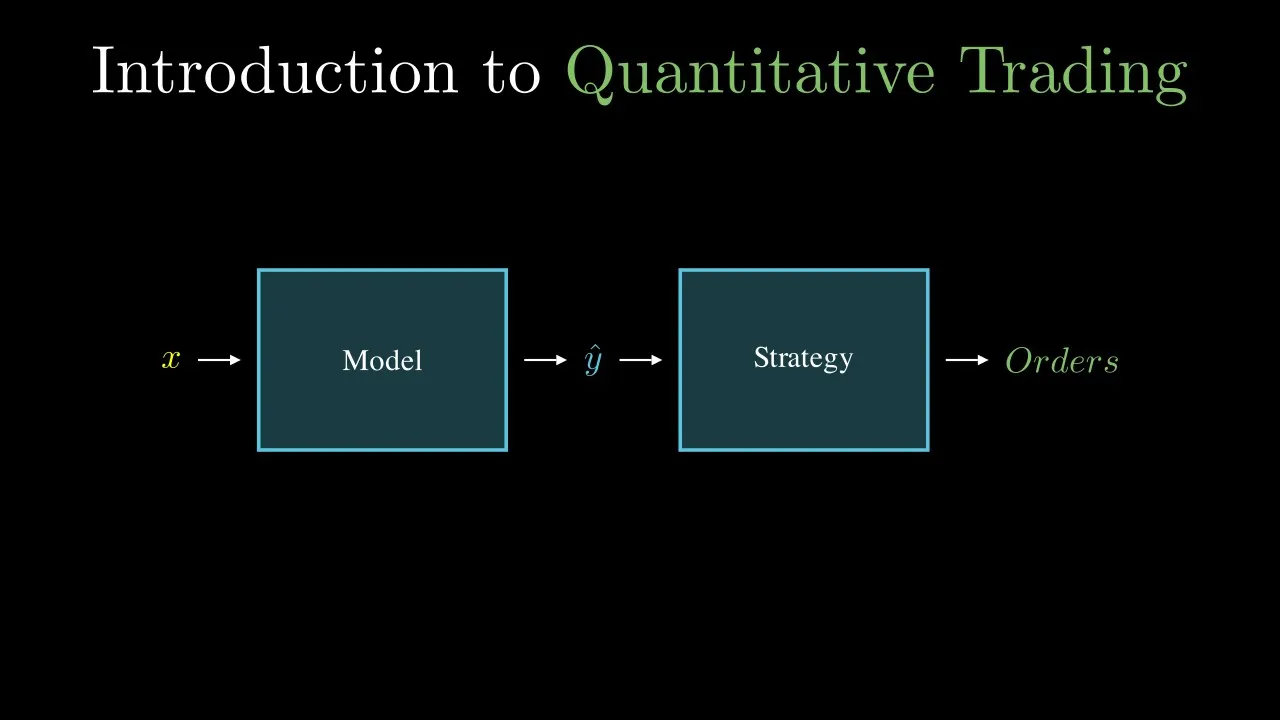
At the heart of quant trading is the model typically a machine learning model. It has both an input and an output. The output is a prediction of a future quantity and is denoted by yhat and the input is denoted by x. There are two types of models, regression and classification. A regression model is a model that predicts a real valued number. It could be predicting the future price, but it could also be trying to predict the the future price difference, which is also called a price delta.
For example, here it is predicting it's going down by $5. or it could be trying to predict the future return represented as a percentage. Returns are unitless and so you're able to compare a model across multiple assets. The other form of model is a classification model which classifies into categories. For example, we could predict if the price is going to go up or down. It also provides an associated probability too.
So here it predicts it's going up with a 75% probability. We call the inputs to a model features and the output it predicts the target. If there's only one feature that's a univaric model can of course use multiple features. Several factors may influence the target, but here's a rule of thumb. The more features you add, the more complexity you introduce. And with complexity comes a higher risk of overfitting to noise and weaker generalization.
That's why in this video we'll focus on univariatic models. They're simple, robust, and less prone to overfitting noise. Advanced models like neuronet networks can even produce multiple outputs. For instance, they might predict returns at several time horizons, the next minute, the next two minutes, and so on, or generate signals for multiple tradable instruments at once. We won't be covering neural networks here. Think of them like driving a Ferrari.
Incredibly powerful, but easy to crash if you don't have experience. They often overfit to noise unless carefully managed. In practice, it's often better to choose simpler models with fewer parameters rather than complex ones. This principle is known as OKAM's Razer. So, what actually goes into a model and what comes out? Typically, the input is a time series, values ordered over time. The model uses past values of the time series to predict a future value in the time series.
The predicted future value is denoted by the red line here. Depending on the model design, it could use the last n values or just the most recent one. In this video, we'll focus on the simplest case using only the last known value as the feature. The model by itself doesn't make money. It generates the edge. And this is where strategy comes in. Strategy is what executes the edge. Both are equally important. You can't make money without a good model and good execution.
The strategy takes the model's predictions and turns them into orders. Think of card counting in blackjack. A system may give you an edge, but if you bet your entire bankroll on the first hand and lose, you execute it poorly. The edge is there, but the but bad execution wipes it out. Other execution details matter, too, like reducing latency to improve order book Q position or avoiding stale prices, but we'll keep those out of scope here.
In this video, we'll explore both the model and the strategy and see how they work to together to form a complete trading algorithm. We'll look at both market making and market taken strategies. Now, I will discuss the core skills needed for quant trading in my humble opinion. The first is econometrics. Econometrics will give you a very good foundation to build upon. It has a rich history of analyzing time series data.
It teaches you how to analyze time series data that changes over time like financial data and helps you identify key patterns and trends in a time series. You'll learn essential concepts like auto reggression, how past values influence the future. Non-stationerity, where the mean and variance of a time series are not constant over time. co co- integration how two non-stationary time series might move together in a stable predictable way.
You could get away with skipping econometrics but it gives you a rich vocabulary for working with time series data. The main limitation is that classical econometric time series models don't scale well to large data sets and make strong assumptions about your data. And this is where machine learning comes in. If there's one skill to focus on, it's this. The power of machine learning is that it learns statistical patterns from historical data without having to explicitly write a complex mathematical formula for it.
Instead of being manually programmed with rules, these models are trained on datadine predictive relationships. For example, the most advanced weather predictions used to rely on intricate hand-coded math formulas. But machine learning models surpass them by learning the best relationships and patterns directly from the data. Machine learning also gives two key advantages. One, scalability. They can scale to large highfrequency data sets such as the orderbook data.
Two, flexibility. It doesn't make any assumptions about your data. You can easily adapt and tweak a model and change what it's optimizing for. Now, strong programming skills are a huge advantage. The better you can code, the less you need to rely on others, and the more control you have over your strategies. Writing latency sensitive algorithms, for example, requires deep knowledge of machine codes, CPUs, memory allocations, operating systems, and networking stacks.
But speed isn't everything. What's often overlooked is systems that run automatically 247 and keep going even when hardware or software errors occur or without performance degrading over time. In practice, reliability is just as important as raw performance. Once you're running multiple trading strategy, scalability becomes critical. You don't want to duplicate code every time you test a new idea. Instead, you need a flexible research API that allows you to build, back test, and deploy strategies without compromising performance.
And the foundation of all this is mathematics. But here's the good news. You don't need to be a math Olympiad winner or a fields medalist to succeed as a quant trader. The level of math involved isn't earthshattering. What you do need is strong mathematical reasoning, the ability to think logically about problems and understand your models on a deeper level, debug issues, and refine strategies with confidence. The math itself is less scary than you might think.
You really need a solid grasp of three key areas. One, linear algebra. Two, multivariable calculus. Three, probability and statistics. The stronger your maths, the more deeply you can understand what's going on under the hood and the more freedom you'll have to innovate. Now, we need to quantify the statistical edge. The statistical edge is quantified as the expected value or EV for short. The expected value tells us on average how much net P&L we can expect per trade.
The higher the EV, the more money we make over the long run. Mathematically, expected value is written as E of X where X is a random variable. In our case, the net P&L of a trade. The net P&L means the profit of a trade after accounting for all costs like transaction fees. Instead of diving straight into the formula, let's build some intuition with a simple game. Imagine a biased coin toss game. You win $1 of its heads with a 55% probability.
You lose $125 if it's tails with a 45% probability. Would you play this game? At first glance, you might say yes. After all, you're winning more often than you lose. However, what if I told you you shouldn't play this game? You might be surprised given that we win more than we lose. If we calculate the expected value of this game, we will see that we lose money on average on each coin toss. So, we shouldn't play this game.
Let's calculate the expected value for this game. The expected value is calculated by the probability of winning multiplied by the value of winning plus the probability of losing multiplied by the value of losing. If we know the values for this so we can plug them in. So now let's plug these values in. And then we see that it becomes 0.55 ultiplied by 1 plus 0.445 ultiplied by -1.25. If we do the calculation we can see that the expected value is negative and it's roughly -1 cent.
This means on average we lose one and a4 cent per toss. The more you play the more you bleed money over time. The key lesson, don't focus only on win rate. Focus on the expected value. The a trading strategy with a 30% win rate can still make money if the winners are larger than uh are large. And a strategy with a 75 70% win rate can still lose money if the losses are too big. Now, let's look at another game. Another coin toss game, but this time you win $35 if it's heads with a 25% probability or you lose $1 if it's tails with a 75% probability.
Should you play this game or not? If you learned your lesson from the previous game, then you know you shouldn't focus purely on the win rate. You should be f uh focusing on the expected value. So, let's do that. Let's calculate the expected value. Again, we know what the variables are, so we can easily plug them in. If we do the calculation, it turns out that we have a tiny positive expected value of roughly 1 and a4 cents.
This means that we should play this game as many times as possible as we'll cumulatively make money. This is indicative of quant trading strategies. Just a tiny tiny edge. where you have a small positive expected value and only win maybe 51% of your trades. But if you make lots of bets, then you can make exceptional returns. We now need to quantify risk adjusted returns. We can informally define it as returns over risk.
Quantifying returns is trivial, but how do you quantify risk? The most common measure of risk is to use standard deviation. And the standard deviation tells you how much variance there is in your data which essentially measures how stable the returns are. The more stable our returns are, the less likely we are to have huge draw downs. We we cannot remove risk to zero, but we can reduce it. More specifically, we define as the expected returns over the standard deviation of returns.
This turns out to be a very common measure called the sharp ratio which is the difference between the expected returns and the risk-free rate over the standard deviation of returns. However, because most quant trading strategies are intraday where we hold onto positions for minutes or hours that we remove the risk-free rate term because we don't hold positions long enough to factor it in. And to to develop the intuition behind the sharp ratio, I've animated uh some simulated sharp ratios.
The sharp ratio is simply a way of measuring return per unit of risk. Here our y-axis is cumulative P&L and the xaxis is time. What I'm showing is how different sharp ratios affect returns. As the sharp increases, the equity curve smooths out. returns become more stable until at very high sharp values it looks like a straight line. Why do we care about reducing risk? One key motivation is leverage. Leverage is multiplying your profits or losses.
So either magnify your losses even bigger if you lose more than you win. With a low sharp, using leverage can quickly wipe you out through liquidations and large draw downs. But the higher the sharp, the more safely you can increase leverage and multiply profits. Now, this doesn't mean you can't make money with a low sharp ratio. Many profitable strategies do, but it does cap how much leverage you can safely allocate.
For example, intraday quant strategies holding positions for just seconds or minutes often have high sharp ratios in the double digits. They may only win 51 to 53% of their trades, but because they make so many small bets with a positive edge, the cumulative returns grow smoothly. At very high sharp levels, the equity curve looks like a straight line, practically printing money. Hopefully, you can see the motivation for reducing risk.
Minimize drawd downs, use leverage safely, and stable returns. We need to discuss simple returns and its biggest limitation. The equation for simple returns is simple. Just take the difference between the current price and previous price and divide by the previous price. However, using simple returns has a limitation in that they are not symmetric. The limitation is best shown with an example. Here is a time series where the price increases by $20 and then decreases by $20.
If we use simple returns, then it goes up by 20% but decreases by -6.6%. So it's asymmetric. We want to make return symmetric. So it goes up and down by the same amount. This is where log returns come in. Log returns is the logarithm of the current price over the previous price. It has a property called time additivity in that you can sum them together to calculate the compound return. So let's go back to the previous example and use log returns instead and see if it solves the problem.
Using log returns instead of simple returns makes our return symmetric. Again, it goes up by $20 and goes down by $20. Using log returns instead, it goes up by 18.2% and goes down by 18.2%. As you can see, it's symmetric now, which plays nicely with our machine learning models and it's easier to reason. Before we go into models, we need to discuss time series. Broadly speaking, there are two types. The first and most common is a regular time series where each data point is recorded at evenly spaced intervals marked by fixed time delta.
For example, in an hourly time series, every data point represents exactly one business hour. In this setup, when we talk about the next data point, we're simply referring to the value at the following hour. However, in high frequency data that the data comes in as an irregular time series and this essentially means that the the delta t between each data point is of a inconsistent size an arbitrary size. So for example, if this was trades, then the trades could come in in the next second, the next minute, the next hour.
And essentially what we're predicting here is rather than say like the the price in the next hour, we're predicting in the next uh data point which we call ticks. Now we need to discuss the concept of auto reggression. Autogression is making predictions of future values from the previous known values which we call lags in ecomtrics. And you probably use auto reggression every day without even noticing. So for example, if you're using chat GPT, this is essentially predicting the the next word from the from the previous words it's generated.
And so it this is why it's called an auto reggressive model because it's making predictions from previous values. And it's exactly the same with a time series. We're interested in making predictions from pre previous known values. Now we're moving into my favorite section, models. In this part, we'll focus on the simplest setup, a one input, one output model. More specifically, we'll be using a linear regression. It's one of the most basic machine learning models, but don't let that fool you.
There's a lot of power in its simplicity. This linear regression model only has two parameters, the weight and the bias. That's it. It multiplies the input with the weight and adds a bias. And that simplicity is what makes it beautiful and powerful because it only has two parameters. One, it has high interpretability. We can actually understand why it makes each prediction. Two, it tends to generalize well, meaning it's less sensitive to noise.
And trust me, there's a lot of noise in trading data. And three, it's calculated very quickly for latency sensitive trading. It only takes three to five CPU cycles to make a prediction. More specifically, we're going to look at an auto reggressive model where we make a prediction from the last known previous value in the time series. In econometrics, this is called an AR1 model. The prediction is the future value of the time series.
And now we'll show examples of using this model. With this auto reggressive linear regression model, we can model the most two fundamental trading behaviors, mean reversion and momentum. I will now show examples of our model fit into these two trading behaviors. So, let's dive right in. Mean reversion is essentially what comes up must come down and what comes down must come up. It hovers around a central tendency. In this example, it's zero.
Here is a log returns time series and you can see it goes from positive to negative and from negative to positive. It's very common to see mean reversion in short time scales like seconds and minutes. So now let's look how we can model mean reversion using our linear regression. Now we need to optimize the weight and the bias to model this mean reversion behavior. We will go into more detail how the parameters are chosen later in the video, but let's just say we've just used a machine learning algorithm to optimize the weight and bias.
Here, our machine learning algorithm has calculated a negative weight and a small tiny bias. The most important detail is that the weight is negative. So, it changes the sign of our lag. So, if it's passed a positive log return, it changes it to a negative log return, then adds a small bias. If passed in a negative log return, then it changes the sign to positive. Now let's see how well our model has done to predict future values by plotting them against each other.
The blue line here shows the actual values we want to predict and the green line shows the predictive values from our model. With even such a simple model, you can see it's done a really good job of capturing this mean reversion behavior. The directional accuracy is 100% accurate. It gets the sign right at every single point. Notice how the predictor values stay very close to the actual ones. And here's the key takeaway.
The negative weight in the model can be interpreted as a mean reversion. Think of it like a rubber band where the price moves away, the negative weight pulls back towards the mean. Now let's see how the same model can also capture the other major trading behavior momentum. This behavior is essentially modeling what goes up stays up and what goes down stays down. As you can see in this log returns time series for the first three data points it remains positive.
So it's trending upwards and then the next three values are negative log returns where it's trending downwards. This persistence in direction is the hallmark of momentum. In financial markets, momentum is one of the most widely studied and traded phenomenas, especially at mediumtime horizons. Let's see how we can model this. Again, using our linear model, we apply machine learning to calculate the optimal parameters.
The key point here is that the this time the weight is positive. So if the current log return is positive, multiplying by the weight keeps the sign positive and then adds a small negative bias. Conversely, if the input is negative, the weight keeps the sign negative. In other words, a positive weight reinforces the existing direction, which is exactly what momentum is about. Now let's see how well these parameters model momentum.
The blue line represents the actual values and the red line shows our predicted values. We can see that the directional accuracy is nearly 100%. And it got the sign wrong at time point.3 where the series transitions from a positive to negative log return. If we look at the distances between the predicted and the actual values, they're minimal. The key point here is that it's the the positive weight doing all the work.
It reinforces the direction of the previous return, which is exactly what momentum is about. So, how did we actually calculate the the weight and the bias? That's what we're going to cover next. This opens up a whole new topic called mathematical optimization, which is simply the process of finding the most optimal par parameters for our model. There are many ways to do this, but we'll focus on the two most important ones.
The first method is closed form solution which gives us an exact analytical answer. This approach is very common in econometrics. If you ever use scikit learns linear regression model, it's actually using a closed form solution under the hood. You can think of it like optimizing the weights in just one line of code, quick and direct. The second method is gradient descent, an iterative approach widely used in machine learning.
Instead of solving everything in one step, it loops over and over, gradually improving the weights until they reach the best values. We'll break each of these down in detail. And here's the mathematics for closed form solution to linear regression, also known as ordinary lease squares. If you've used linear regression in Mat Lab, Mathematica or the linear regression class in Scikitlearn, then this is the exact equation being used to solve the problem.
The beauty of of OS is that it can be calculated in just one line of code. It gives very good approximations, but it has one big limitation. It doesn't scare well to large data sets. It works perfectly for small data sets, but when you're dealing with terabytes of data, it becomes inefficient to load everything into memory and perform massive matrix calculations. With high frequency data, we can collect terabytes of data daily.
So, it quickly becomes infeasible to rely on ordinary squares alone. And this is where gradient descent comes into play. Instead of solving everything at once, gradient descent loops over the data and incrementally improves the parameters using small batches of training data at a time. The weight update rule is simple. Take the current weight and subtract the partial gradient. The partial gradient is just the derivative of the loss function with respect to the weight.
And the loss function is something we as modelers get to choose. It defines how we measure error. An important hyperparameter is the learning rate usually denoted by the Greek letter eta which controls how big each update step is. Too large and you overshoot the optimal solution and too small the training becomes painfully slow. The beauty of gradient descent is in its flexibility. We can choose different loss functions and sometimes there's real alpha in designing new and creative ways to define that loss function.
I I will now illustrate how gradient descent works so you have an understanding of its mechanics. And here's gradient descent in action. Here we're looking at the convex loss function like mean squared error. The goal of gradient descent is to find the minimum of this function, the point where the error is small as possible. At each step, the algorithm calculates the gradient, the slope of the function, and then takes a step in the opposite direction of the gradient.
Since this function is convex, there's only one global minimum. At that minimum, we found the best parameters for our model. When designing custom loss functions, they are often non-convex. That means instead of one unique minimum, there are many local minima and even saddle points. The optimizer's goal isn't to find the perfect global minimum. That's usually impossible. But to land in a good local minimum that performs well.
Sometimes it may converge to a poor region, but techniques like stochastic gradient descent or momentum help uh escape bad spots. In practice, the aim is not perfection, but finding a solution that generalizes well. In this example, it finds a local minima that is a good approximation of the global minima. As we've said before, execution is just as important as the edge itself. If you have a great model but poor execution, there's no real alpha.
We're just going to focus on the strategy exclusively. How we take the model's predictions and translate them into actual orders. Of course, in practice, there are many nuances. Things like minimizing latency to get better prices and Q positions, which become critical if you're trading on second or minute time horizons. But since this is just an introduction, we'll set aside those low-level execution details and focus purely on the strategy.
The taxonomy of quant trading strategies can be divided into two broad types, making and taking. Making means adding liquidity to the order book. In this case, you're often rewarded either through rebates or with such low transaction fees that it becomes feasible to trade at a second or minute level time horizon. Taking on the other hand is removing liquidity from the order book. Here you typically pay higher transaction fees.
That makes very short horizon trading less attractive because even if your back test shows strong gross P&L, those fees can push your net P&L negative. Of course, this is just a loose taxonomy. In practice, many strategies combine both making and taking depending on the situation. We'll dig into each more detail next. Before we jump into strategies, we need to cover the fundamentals of the order book. The order book is the heart of a financial market.
It represents the global supply and demand. Market makers add limit orders to provide liquidity. Market orders remove liquidity from the book. Having access to the order book can give you a predictive edge. The book itself contains two sides. bids, which are buy orders and asks, sell orders. These are organized into levels. At the very top of the book, you always see the best bid and best ask, the highest price someone is willing to buy and the lowest price someone is willing to sell, along with the available quantities at those levels.
And this isn't static. Prices and quantities are constantly shifting as trades happen and orders flow in. The order book is a live reflection of the market micro structure in real time. An important measure of the order book is the spread. The difference between the best bid and the best ask. As a rule of thumb, less liquid markets have wider spreads while highly liquid markets usually have narrower spreads. The spread is also a hidden cost for taking strategies.
If you buy at the ask and immediately sell at the bid, you lose the spread. That's why market makers, also called liquidity providers, earn money by continuously buying at the bid and selling at the ask. Spreads can also widen during volatile or uncertain conditions as liquidity providers demand more compensation for risk. In short, the spread is the gap between supply and demand. It reflects liquidity costs and risk.
In this example, the spread is 3 cents as it's the difference between 115 and 113. An important measure to predict from the order book is the mid price. The mid price is simply the average of the best bid and the best ask. It's very important for making strategies because you need to know where the mid price is moving in order to bias your quotes accordingly. You might wonder why not just use the last trade price. The reason is because of the bid ask bounce.
Trades tend to alternate between the bid and the ask which adds unnecessary noise to the time series. That's why the mid price gives a cleaner signal. The mid price for this order book is 113 12 cents and the bid ask bounce is more apparent when it's visualized. So let's do that. Here we have a time series of last traded prices. And notice how it bounces back and forth between the bid and the ask. This back and forth creates extra variance in the series.
Nor is that doesn't really reflect true market movement. Now, if instead we plot the mid price for each point in time, the picture changes. The mid price stays stable between trades. No artificial noise from the spread. That's why the mid price is usually preferred in modeling because it gives a cleaner, less noisy signal. Let's walk through what happens when a market order comes in and how it affects the order book.
Suppose we send a buy market order for two contracts. Since this is a buy, we need a seller. So, the order crosses the ask side of the book. Market orders are always filled against the opposite side. So here the order is matched against the best ask price. Once it's filled, the quantity at that price level is reduced to reflect the liquidity has been taken away. That's why market orders are called taken while limit orders are called making.
For example, if the top of the book is shown 115 with three contracts available and we buy two with a market order, the order book updates to show just one contract left at that price. Sometimes if the market orders larger than what's available at the best price eats through multiple levels of the book that effect is called slippage. Now let's see what happens when we send a larger market order say 10 contracts at the best best ask price 115 there only three contracts available.
Our order takes those out but we still have seven left to fill. So the order walks the book and crosses into the next level at 116. This is called slippage where we aren't able to buy everything at the best ask. So part of the order got filled at worst prices. In this case, we've bought three contracts at 115 and the rest at higher levels. Notice what happens next. The mid price shifts upward. Since the best ask has moved from 115 to 117, that also means the spread has widened.
When this happens in real markets, market makers react. They might raise their best bids to follow the move or refill liquidity at the old price levels. And this purely depends on models and algorithms. A taken strategy uses market orders, which means you're guaranteed execution, but not the exact price. They're typically deployed for longer time frames from hours to days or even weeks. Because the net P&L is usually negative on a second or minute level time frame because of the high transaction fees and spread.
When building a taken strategy, there's two key decisions. timing, when to enter an exit trade, and sizing, how much to trade each time. We'll break down both of these next. The timing of a taken strategy can be loosely grouped into two approaches. Timebased timing, where trades are entered or exited strictly at set intervals. This pairs naturally with time series models since they generate predictions at fixed horizons. predicate based timing where trades are triggered only when a specific condition is met.
For example, if our model predicts a value above or below a certain threshold, that predicate determines the entry. We'll dive deeper into both of these approaches next. Timebased timing means opening and closing trades on a fixed schedule. For example, in a daily time series, the model makes a prediction each day. Based on that prediction, we open a position, then close it the next day. If the model predicts the same direction on the consecutive days, we don't always close the the position.
Instead, we could hold the position and scale it up depending on the risk profile of the strategy. This approach fits naturally with time series models since every data point corresponds to a specific time interval. Now you might be asking what about stop losses or take profit levels. These can be added but only if they increase expected value. Always back test first. For example, in a mean reversion model, adding a stop-loss could actually reduce performance since we expect prices to bounce back.
Now let's induce the idea of frequency scaling. Suppose we open and close positions every 12 hours. That's only two trades a day, one to open and one to close. If our edge is small, that's not much opportunity to really exploit a tiny edge. We want to maximize the number of bets. One way to do that is by increasing the resolution of the time series. For example, instead of 12-hour intervals, we move to 1 hour intervals.
Now, each data point represents an hour. We still hold trades for 12 hours, but within that window, we're making many smaller trades over 12 hours. That's 24 trades. Every hour, we adjust by opening or scaling up and then reducing or closing. Because everything happens at fixed intervals, we can control risk and make sure our position size never exceeds a cap. Now, what if the model predicts long one hour and short the next?
In that case, you'd need positions in both directions. Some brokers and exchanges support this through hedge mode, while others require you to set up a sub account to run long and short simultaneously. As you can see in this example, the model is predicting where the price will be 12 hours into the future. But instead of waiting the full 12 hours to act, we place bets every hour. Each hour, we adjust either increasing or decreasing our position size in each direction while still anchoring everything to that 12-hour forecast. predicate based timing means we don't trade on every single prediction.
Instead, we filter the model's output and only place trades when a specific condition, a predicate, is satisfied. For example, let's say we only go long if the model's predicted future log return is greater than or equal to 0.01 and only go short if it's less than or equal to minus0.01. If the prediction falls in between, we simply don't trade. For example, for a binary classification model, we might only want to trade long if the probability is greater or equal to 60% and only trade short if it's lower than or equal to 40%.
The idea here is to boost the expected value of the strategy by ignoring weak or noisy predictions and only acting on stronger signals. But remember, you have to back test. Sometimes filtering too aggressively can reduce opportunities and actually hurt EV. The other important detail of a taking strat is trade size. If we oversize our trades, we risk severe draw downs, liquidation, or even bankruptcy. The intuition is simple.
Bet small, bet often. With high frequency strategies, losing a single trade shouldn't derail the system. In fact, some of the best quant strategies only win 51 to 53% of the trades. If your edge is that small, oversizing is a guaranteed way to blow up. Now, in practice, you would also account for market impact, how your own trades move the price, but that's outside the scope of this intro. There are classical methods like the Kelly criterion, but those don't adapt to your model's predicted edge.
For our purposes, we'll keep things simple and focus on trade sizes that scale directly with models predictions. We can roughly group sizing methods into three categories. Constant, where the trade size is always the same. peacewise linear that scale trade size proportionally linearly with the model's prediction and then nonlinear and we'll go into detail for each one. Constant trade size means we always trade the same size no matter what the model predicts.
It's a great baseline especially for timebased strategies. For example, if we're trading every hour and holding each position for 20 hour 24 hours, we could have up to 24 concurrent trades, we'll divide our allocated capital across those 24 slots. If we want, we can also apply a leverage factor on top. In practice, our signed trade size is just the sign of our model's prediction multiplied by that constant. I recommend starting with constant sizing when back testing.
It's simple, easy to interpret, and gives you a clean benchmark. Once you've tested that, you can explore more advanced sizing methods to see if they increase your expected value. Here's an example of a peace-wise linear sizing method. Instead of always trading the same size, we scale our trade size with the strength of the model's prediction. We don't want position sizes to blow up, so we keep them bounded. A simple way to do this is with the hard tangent function borrowed from deep learning.
It acts like a linear function in the middle but clips the values at an upper and lower limit. In trading terms, our sign trade size is just the maximum trade size multiplied by the hard tangent of the model's prediction. That way, the stronger predictions get bigger trades and weaker predictions get smaller trades. And nothing ever exceeds our set bounds. Now let's look at nonlinear sizing methods. Here the signed trade size is the maximum trade size multiplied by the tangent of the model's prediction.
It works a lot like hard tangent but instead of sharp cutffs the tangent function gives us a smoother more gradual scaling of trade sizes as the predictions increase or decrease. That smoothness makes it more sensitive to small changes in prediction strength while keeping trade sizes naturally bounded. And since tangent is a differentiable everywhere in its range, it also plays nicely if you're optimizing parameters with gradient-based methods.
This animation shows our nonlinear trade sizing using tanh. Here the maximum trade size is 100 and you can see it's smoothly bounded between minus 100 and 100. For making strategies there are two key parameters spread and bias. The spread is the difference between our bid and ask price. Essentially how much profit we expect to capture per trade. The bias also called skew adjusts our prices to make our bid or ask more likely to be filled.
This ensures we have a position in the right direction of our model. Spread is the profit we aim to capture between our bid and ask price. For example, if the mid price is $5 and want a $2 spread, you place a limit order to buy at $4 and a limit order to sell at $6. This means we buy at four and sell at $6. So, make a $2 profit. When a limit order is executed, we say it is filled. making strategies are harder to back test because of how you simulate how limit orders are filled or not, which is out of the scope of this introduction.
For example, if the price is at $4, how do you know the bid is filled or not? There's a trade-off when setting the spread. If the spread is too wide, you maximize your potential profit but risk never getting filled. For example, if you set a $4 spread with a bid at three and uh an ask at seven, you're aiming for a big margin. But if no one trades at those prices, your profits stay unrealized, effectively zero. If the spread is too narrow, you have more fills but risk adverse selection, taking positions in the wrong direction.
This can negatively impact our expected value. For example, if we drop if the price drops down to $3 and a half and our bid is filled at $4.75, we we so we have a long position in the wrong direction. This is adverse selection. A way to fix adverse selection is by biasing your prices. Biasing is adjusting prices to tilt your position in a certain direction. This is where the alpha lies, how you skew your quotes based on your model's prediction.
Importantly, biasing doesn't change the spread size, only the placement of the bid and ask relative to the mid price. For example, suppose we quote a $20 spread with a bid at 90 and ask at 110. If our model predicts the mid price will rise, we bias upward, shift both quotes higher while keeping the $20 spread intact. Now our bid is more likely to be hit, giving us a long position aligned with our prediction. In practice, this is where the edge comes from.
Systematically biasing quotes in line with a model's prediction where the mid price is moving and is often driven by order book imbalances. We can bias more aggressively by moving the bid closer to the mid price and the ask further away, making it more likely to accumulate a long position. You might want to shift by a constant size or proportional to the model's predicted value. There's no right or wrong answer here.
Only back testing will tell. If your model has a tiny edge, which is common for predictions in the second or minutes, then you want to ensure you trade as much as possible. So you might want to aggressively bias your prices. If the model predicts the mid price will fall, we bias in the opposite direction, shifting both bid and ask lower. Again, the spread size is unchanged, but we're we're skewing fills towards the short side.
Here we're quoting our bid at 85 and our ask at 105. Our spread hasn't changed. Just it's more likely for ask to be lifted. Also, we can aggressively bias the other way. So, it's more likely to accumulate a short position. The bias is dynamically changing based on the model's prediction. And also, the spread could be dynamically adjusting based on the volatility or inventory risk. The model is typically predicting the midpric delta, how much the mid price is going to move by.
That wraps everything up. Hopefully, you found this educational. You should now understand how a statistical edge is both created and executed with the model generating the edge and the strategy executing it in the market. Of course, this was just an introduction. There's a lot more depth to explore, more advanced models, more sophisticated execution, and even strategies that combine multiple models into portfolios. I'd love to hear your feedback, so please leave a comment.
It really helps me to improve and shape future videos. And and if there's any specific topic you'd like me to cover next, let me know. Thanks for watching, and please like and subscribe.
The words are the caption track's own and nothing is reworded or re-transcribed. Paragraph breaks are placed between sentences so the text reads as prose.
Free tools for your own script: paste a draft and see where it stands before you record it.
Paste your draft and see where viewers are likely to drop off, with a rewrite for each weak line.
Paste the first 30 seconds of your own draft for a hook score and rewrites.
Check your draft against YouTube's advertiser-friendly guidelines before you record it.
Read this channel's public videos and transcripts, and download a writing brief for it.